The variational principle: helium ground state and the hydrogen molecule ion

Perturbation theory needs a nearby solvable problem and a small parameter. Many important problems have neither. The helium atom's electron repulsion is not small, and no textbook Hamiltonian is close to a molecule. For ground states there is a different method that needs nothing but a good guess. It rests on a theorem so simple that its proof takes three lines, yet it underlies nearly all of computational chemistry and much of condensed-matter physics. This lesson proves the theorem, applies it to the helium ground state and to the simplest molecule, \(\text{H}_2^+\), and shows how it explains the chemical bond.

The variational principle

Let \(H\) be a Hamiltonian with ground-state energy \(E_{\text{gs}}\). For any normalized state \(\psi\), whatever its form,

The proof: expand \(\psi\) in the (unknown) eigenstates of \(H\), \(\psi = \sum_n c_n\psi_n\) with \(H\psi_n = E_n\psi_n\) and \(\sum_n|c_n|^2 = 1\). Then \(\langle H\rangle = \sum_n E_n|c_n|^2\), and since every \(E_n \ge E_{\text{gs}}\), \(\langle H\rangle \ge E_{\text{gs}}\sum_n|c_n|^2 = E_{\text{gs}}\). Equality holds only if \(\psi\) is the ground state. The principle turns the search for a ground state into a minimization: choose a trial function with adjustable parameters, compute \(\langle H\rangle\) as a function of them, and minimize. The result is always an upper bound, and better trial functions give lower, more accurate bounds.

Two further facts make the method more powerful than it looks. First, the energy is much less sensitive to errors in the trial function than the function itself: if \(\psi\) differs from the true ground state by a small amount of order \(\epsilon\), \(\langle H\rangle\) differs from \(E_{\text{gs}}\) only by order \(\epsilon^2\), because the true ground state makes \(\langle H\rangle\) stationary. A mediocre wave function can give an excellent energy. Second, if the trial function is constrained to be orthogonal to the true ground state, for instance by symmetry, the same argument gives an upper bound on the first excited state. A trial function that is odd under parity, for a symmetric potential, bounds the lowest odd state.

A first test: hydrogen with the wrong shape

To see the method at work, apply it to a problem whose answer we know, using a deliberately poor trial function. For hydrogen, try a Gaussian, \(\psi = (2b/\pi)^{3/4}e^{-br^2}\), which has the wrong behavior both at the origin (no cusp) and at large distance (it falls off too quickly). A short calculation in atomic units gives \(\langle T\rangle = 3b/2\) and \(\langle V\rangle = -2\sqrt{2b/\pi}\) hartree. Minimizing over \(b\) gives \(b = 8/9\pi\) and \(E = -(8/3\pi)(13.6\ \text{eV}) = -11.5\) eV, about 85 parts in 100 of the true binding. A function with the wrong shape still captures most of the energy. Quantum chemistry codes in fact build molecular orbitals from sums of Gaussians, because their integrals are easy, and use enough of them to fix the shape.

Helium: screening as a variational parameter

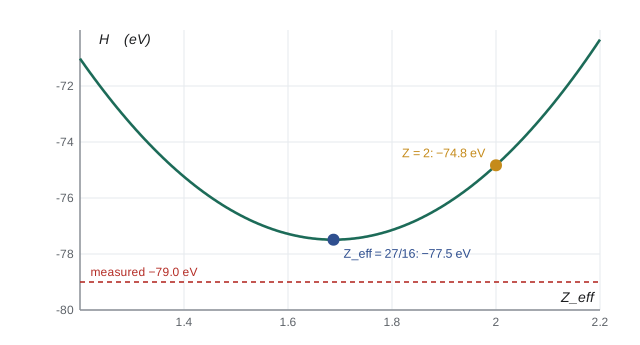
For helium, start from the product of two hydrogenic ground-state orbitals with nuclear charge \(Z\), \(\psi_0 = (Z^3/\pi a^3)e^{-Z(r_1 + r_2)/a}\). This is the exact ground state without the repulsion, and with \(Z = 2\) it gives the first-order energy \(-74.8\) eV of lesson 1. But each electron partly shields the nucleus from the other, so a better trial function lets the charge in the orbitals be a parameter \(Z_{\text{eff}}\), different from the true nuclear charge \(Z = 2\) in the Hamiltonian. The expectation value of the Hamiltonian, in hartrees, is

The first term is the kinetic energy of two electrons in orbitals of charge \(Z_{\text{eff}}\); the second is their attraction to the true nucleus of charge \(Z\); the third is the repulsion, \(\tfrac58 Z_{\text{eff}}\) hartree, the same integral as in first-order perturbation theory but now with the smaller orbitals' charge. Setting the derivative to zero gives

Each electron sees the nucleus screened by about 5/16 of the other electron's charge, and the energy improves from \(-74.8\) to \(-77.5\) eV, within 2 parts in 100 of the measured \(-79.0\) eV. Better trial functions do even better. Hylleraas in 1929 added the interelectron distance \(r_{12}\) as a variable, building into the wave function the tendency of the electrons to avoid each other; with just a few terms he reached \(-78.98\) eV. Modern calculations with thousands of terms give the nonrelativistic helium energy to more than twenty significant figures, and after relativistic and QED corrections agree with the measured ionization energy, the most precise test of quantum mechanics in a three-body system.

The hydrogen molecule ion

The simplest molecule is \(\text{H}_2^+\): two protons sharing one electron. Treating the protons as fixed at separation \(R\), an approximation justified by their mass, which makes them move far more slowly than the electron (the Born–Oppenheimer approximation of 1927), the electron's Hamiltonian is

where \(r_1\) and \(r_2\) are the distances from the electron to the two protons, and the trial function is a linear combination of hydrogen ground-state orbitals centered on each proton, the LCAO approximation (linear combination of atomic orbitals). It is the natural guess: when the electron is near one proton, it should look like a hydrogen atom. The calculation needs three integrals, all expressible in closed form: the overlap \(S = \langle\psi_0(r_1)|\psi_0(r_2)\rangle = e^{-R/a}(1 + R/a + R^2/3a^2)\), the direct integral \(D = a\langle\psi_0(r_1)|1/r_2|\psi_0(r_1)\rangle\) and the exchange integral \(X = a\langle\psi_0(r_1)|1/r_1|\psi_0(r_2)\rangle\). Adding the proton–proton repulsion \(e^2/4\pi\varepsilon_0R\), the total energy in rydbergs is

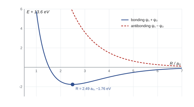
For bonding to occur, \(E(R)\) must dip below \(-1\) rydberg, the energy of a hydrogen atom and a distant proton. It does. The program finds the minimum at \(R = 2.49a = 0.132\) nm with a binding energy of 1.76 eV. The exact solution of the \(\text{H}_2^+\) problem, possible numerically because the potential separates in elliptic coordinates, gives \(R = 2.00a\) and 2.79 eV. The simple trial function proves that the molecule is bound, with an upper bound on the energy and a reasonable bond length, and improving it (for instance by letting the orbital charge vary, as for helium) brings the numbers close to exact.

import math
Ry = 13.605693            # eV; atomic-unit formulas below give energies in rydbergs or hartrees as noted

def golden_min(f, a, b, tol=1e-10):
    g = (math.sqrt(5) - 1) / 2
    c, d = b - g * (b - a), a + g * (b - a)
    while b - a > tol:
        if f(c) < f(d): b, d = d, c; c = b - g * (b - a)
        else: a, c = c, d; d = a + g * (b - a)
    x = (a + b) / 2; return x, f(x)

# 1. hydrogen with a Gaussian trial function exp(-b r^2): <H> = 3b/2 - 2 sqrt(2b/pi) hartree
EH = lambda b: 1.5 * b - 2 * math.sqrt(2 * b / math.pi)
b, E = golden_min(EH, 0.01, 2.0)
print(f"hydrogen, Gaussian trial: best b = {b:.4f} / a0^2, E = {E * 2 * Ry:.3f} eV (exact -13.606 eV, ratio {E * 2:.4f})")

# 2. helium with screened hydrogenic orbitals: <H> = Zeff^2 - 2 Z Zeff + (5/8) Zeff hartree, Z = 2
Z = 2
EHe = lambda z: z * z - 2 * Z * z + 5 / 8 * z
z, E = golden_min(EHe, 1.0, 2.0)
print(f"helium, screened orbitals: Zeff = {z:.4f} (27/16 = {27 / 16:.4f}), E = {E * 2 * Ry:.2f} eV (measured -79.00 eV)")
for zz in (2.0, 1.8, 1.6875, 1.5):
    print(f"   Zeff = {zz:6.4f}: <H> = {EHe(zz) * 2 * Ry:7.2f} eV")
# ionization energy of helium: E(He+) = -Z^2/2 hartree = -54.42 eV
print(f"   predicted first ionization energy: {-54.42 - E * 2 * Ry:.2f} eV (measured 24.59 eV)")

# 3. the hydrogen molecule ion H2+ with the LCAO trial function psi_1(r1) + psi_1(r2)
def H2plus(x):
    """Energy in rydbergs (relative to separated H + p is -1) at proton separation x = R / a0."""
    S = (1 + x + x * x / 3) * math.exp(-x)
    D = (1 / x - (1 + 1 / x) * math.exp(-2 * x))        # direct integral a <psi1|1/r2|psi1>
    X = (1 + x) * math.exp(-x)                          # exchange integral a <psi1|1/r1|psi2>
    return -1 + 2 / x - 2 * (D + X) / (1 + S)
x, E = golden_min(H2plus, 1.0, 5.0)
print()
print(f"H2+ LCAO: equilibrium R = {x:.3f} a0 = {x * 0.0529177:.4f} nm, binding {-(E + 1) * Ry:.2f} eV")
print("   (exact: R = 2.00 a0 = 0.106 nm, binding 2.79 eV)")
for xx in (1.0, 1.5, 2.0, 2.5, 3.0, 4.0, 6.0):
    print(f"   R = {xx:3.1f} a0: E + 13.6 eV = {(H2plus(xx) + 1) * Ry:+6.3f} eV")

hydrogen, Gaussian trial: best b = 0.2829 / a0^2, E = -11.549 eV (exact -13.606 eV, ratio -0.8488)
helium, screened orbitals: Zeff = 1.6875 (27/16 = 1.6875), E = -77.49 eV (measured -79.00 eV)
   Zeff = 2.0000: <H> =  -74.83 eV
   Zeff = 1.8000: <H> =  -77.14 eV
   Zeff = 1.6875: <H> =  -77.49 eV
   Zeff = 1.5000: <H> =  -76.53 eV
   predicted first ionization energy: 23.07 eV (measured 24.59 eV)

H2+ LCAO: equilibrium R = 2.493 a0 = 0.1319 nm, binding 1.76 eV
   (exact: R = 2.00 a0 = 0.106 nm, binding 2.79 eV)
   R = 1.0 a0: E + 13.6 eV = +5.759 eV
   R = 1.5 a0: E + 13.6 eV = +0.136 eV
   R = 2.0 a0: E + 13.6 eV = -1.463 eV
   R = 2.5 a0: E + 13.6 eV = -1.764 eV
   R = 3.0 a0: E + 13.6 eV = -1.608 eV
   R = 4.0 a0: E + 13.6 eV = -1.003 eV
   R = 6.0 a0: E + 13.6 eV = -0.247 eV

Why the bond forms

The physics of the bond is visible in the trial function. The symmetric combination \(\psi_0(r_1) + \psi_0(r_2)\) piles up electron probability in the region between the protons, where it is attracted to both at once and where its wave function curves less, lowering its kinetic energy. The antisymmetric combination \(\psi_0(r_1) - \psi_0(r_2)\), which has a node midway between the protons, removes electron density from that region; its energy lies above \(-1\) rydberg at every separation, so it is an antibonding orbital. The exchange integral \(X\), which exists only because the electron can be near either proton, is what makes the difference. This is the quantum mechanical origin of the covalent bond, first worked out for the neutral \(\text{H}_2\) molecule by Walter Heitler and Fritz London in 1927. In \(\text{H}_2\) two electrons occupy the bonding orbital with opposite spins, the singlet of lesson 4, and the bond energy is 4.5 eV. Linus Pauling built a theory of chemical bonding on these ideas in the 1930s, and Robert Mulliken's molecular-orbital theory, which uses LCAO orbitals spread over the whole molecule, earned him the 1966 Nobel Prize in Chemistry.

The variational method in practice

Real calculations take the trial function to be a linear combination of many fixed basis functions, \(\psi = \sum_i c_i\phi_i\). Minimizing \(\langle H\rangle\) over the coefficients turns into a matrix eigenvalue problem, \(\mathbf H\mathbf c = E\,\mathbf S\mathbf c\), with \(H_{ij} = \langle\phi_i|H|\phi_j\rangle\) and overlap matrix \(S_{ij} = \langle\phi_i|\phi_j\rangle\). This is the Rayleigh–Ritz method, named for Lord Rayleigh (1870s) and Walther Ritz (1908). Its lowest eigenvalue bounds the ground state, and its higher eigenvalues bound the excited states in order, a result known as the Hylleraas–Undheim–MacDonald theorem. The exact diagonalization of the quartic oscillator in lesson 6 was just this method with oscillator basis functions. For many electrons, the Hartree–Fock method uses a single Slater determinant as the trial function and optimizes its orbitals, and density functional theory, for which Walter Kohn shared the 1998 Nobel Prize in Chemistry, rests on a variational principle for the electron density. Both are run every day on supercomputers to design catalysts, drugs and battery materials.