Addition of angular momenta and Clebsch–Gordan coefficients

An electron in an atom has orbital angular momentum \(\mathbf L\) and spin \(\mathbf S\). A helium atom has two electrons, each with its own orbital angular momentum and spin. A deuteron is a proton and a neutron, each of spin one-half. In all of these, the quantity conserved by the full Hamiltonian is usually not any single angular momentum but their sum, and the energy levels are labeled by the total. This lesson answers a question that sounds simple: if one system has angular momentum quantum number \(j_1\) and another has \(j_2\), what values can the total take, and how are the states of definite total built from the states of the parts? The answer, with its coefficients named after Alfred Clebsch and Paul Gordan, who studied the corresponding problem in nineteenth-century invariant theory, is used in every corner of atomic, nuclear and particle physics.

The rules for adding

Let \(\mathbf J_1\) and \(\mathbf J_2\) be two commuting angular momenta, each obeying the standard algebra, and let \(\mathbf J = \mathbf J_1 + \mathbf J_2\). Because each component of \(\mathbf J_1\) commutes with each component of \(\mathbf J_2\), the sum also satisfies \([J_x, J_y] = i\hbar J_z\), so everything proved in PHYS-372 about angular momentum applies to \(\mathbf J\): its states can be labeled \(|J, M\rangle\) with \(J^2 = \hbar^2 J(J+1)\) and \(J_z = M\hbar\). The question is which \(J\) values occur. Two facts settle it.

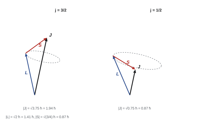
This is the quantum version of adding two vectors of fixed lengths: the total can be anything from the difference to the sum, but only in integer steps. Two spin one-half particles give \(S = 1\) or \(0\); orbital \(\ell = 1\) with spin one-half gives \(j = 3/2\) or \(1/2\); two \(\ell = 1\) electrons give \(L = 2, 1\) or \(0\). In the vector model, the two angular momenta precess about their resultant, which is fixed in length and direction, while their individual \(z\) components are not definite.

Two spin one-half particles

The simplest case is the most important. With two spin one-half particles there are four product states, \(|{\uparrow\uparrow}\rangle, |{\uparrow\downarrow}\rangle, |{\downarrow\uparrow}\rangle, |{\downarrow\downarrow}\rangle\). The state \(|{\uparrow\uparrow}\rangle\) has \(M = 1\) and must be \(|1, 1\rangle\). To find \(|1, 0\rangle\), apply the total lowering operator \(S_- = S_{1-} + S_{2-}\), using \(S_-|1, 1\rangle = \hbar\sqrt2\,|1, 0\rangle\) on the left and \(S_{i-}|{\uparrow}\rangle = \hbar|{\downarrow}\rangle\) on the right:

Lowering once more gives \(|1, -1\rangle = |{\downarrow\downarrow}\rangle\). These three states form the triplet. The fourth state must have \(M = 0\) and be orthogonal to \(|1, 0\rangle\), so it is

the singlet. One can check directly that \(S^2\) annihilates it, using \(S^2 = S_1^2 + S_2^2 + 2\mathbf S_1\cdot\mathbf S_2\) and the identity \(2\mathbf S_1\cdot\mathbf S_2 = S_{1+}S_{2-} + S_{1-}S_{2+} + 2S_{1z}S_{2z}\). The triplet states are symmetric under exchange of the two spins and the singlet is antisymmetric, a fact that becomes crucial for identical particles in lesson 4. The same identity gives a result used again and again: \(\mathbf S_1\cdot\mathbf S_2 = \tfrac12(S^2 - S_1^2 - S_2^2)\), which equals \(+\tfrac14\hbar^2\) in the triplet and \(-\tfrac34\hbar^2\) in the singlet. Any interaction proportional to \(\mathbf S_1\cdot\mathbf S_2\), such as the hyperfine coupling of the electron and proton in hydrogen, splits the triplet from the singlet.

Clebsch–Gordan coefficients

In general, each state of definite total angular momentum is a linear combination of product states with the same \(M\):

The coefficients are the Clebsch–Gordan coefficients. They can always be found as above: start from the top state \(|j_1 + j_2, j_1 + j_2\rangle = |j_1 j_1\rangle|j_2 j_2\rangle\), lower repeatedly to fill out the highest \(J\), then construct the top state of the next \(J\) by orthogonality, lower again, and so on. With the standard phase convention, introduced by Condon and Shortley in 1935, all the coefficients are real, and the change of basis they define is an orthogonal matrix. So the coefficients satisfy two sets of orthogonality relations, and the inverse expansion uses the same numbers:

For \(\ell = 1\) and \(s = \tfrac12\), the states that matter for the \(2p\) level of hydrogen, the results are

where \(|m_\ell, m_s\rangle\) labels the product states. A \(2p_{1/2}\) electron with \(m_j = \tfrac12\) is, two thirds of the time, found with \(m_\ell = 1\) and spin down. Such coefficients determine the relative strengths of spectral lines and of the Zeeman components in lesson 7. Tables of Clebsch–Gordan coefficients appear in every reference book on particle physics, and they can also be computed from a closed formula due to Giulio Racah (1942), which the program below implements.

from fractions import Fraction as F
from math import factorial, sqrt

def cg(j1, m1, j2, m2, J, M):
    """Clebsch-Gordan coefficient <j1 m1; j2 m2 | J M> by Racah's formula (half-integers as Fractions)."""
    if m1 + m2 != M or not (abs(j1 - j2) <= J <= j1 + j2) or abs(M) > J or abs(m1) > j1 or abs(m2) > j2: return 0.0
    f = lambda x: factorial(int(x))
    pre = (2 * J + 1) * f(J + j1 - j2) * f(J - j1 + j2) * f(j1 + j2 - J) / f(j1 + j2 + J + 1)
    pre *= f(J + M) * f(J - M) * f(j1 - m1) * f(j1 + m1) * f(j2 - m2) * f(j2 + m2)
    s = 0.0
    for k in range(0, int(j1 + j2 + J) + 2):
        d = [k, j1 + j2 - J - k, j1 - m1 - k, j2 + m2 - k, J - j2 + m1 + k, J - j1 - m2 + k]
        if all(x >= 0 for x in d):
            s += (-1) ** k / (f(d[0]) * f(d[1]) * f(d[2]) * f(d[3]) * f(d[4]) * f(d[5]))
    return sqrt(pre) * s

h = F(1, 2)
print("Two spin one-half particles: coefficients <m1 m2 | S M>")
for S in (1, 0):
    for M in range(S, -S - 1, -1):
        terms = [(m1, M - m1, cg(h, m1, h, M - m1, S, M)) for m1 in (h, -h) if abs(M - m1) <= h]
        txt = '  '.join(f"{c:+.4f}|{'u' if m1 > 0 else 'd'}{'u' if m2 > 0 else 'd'}>" for m1, m2, c in terms if abs(c) > 1e-12)
        print(f"  |S={S}, M={M:+d}> = {txt}")

print()
print("Orbital l = 1 with spin 1/2: |j, mj> in terms of |ml, ms>")
for J in (F(3, 2), F(1, 2)):
    M = F(1, 2)
    terms = [(ml, M - ml, cg(1, ml, h, M - ml, J, M)) for ml in (1, 0, -1) if abs(M - ml) <= h]
    txt = '  '.join(f"{c:+.4f}|ml={ml:+d},ms={'+' if ms > 0 else '-'}>" for ml, ms, c in terms if abs(c) > 1e-12)
    print(f"  |j={J}, mj=+1/2> = {txt}")

print()
print("Checks: completeness and dimension counting")
for j1, j2 in ((h, h), (1, h), (1, 1), (F(3, 2), 1)):
    total = 0; ok = True
    Js = []
    J = abs(j1 - j2)
    while J <= j1 + j2: Js.append(J); total += int(2 * J + 1); J += 1
    # orthonormality: sum over m1 of CG^2 for fixed J, M equals 1
    for J in Js:
        for k in range(int(2 * J + 1)):
            M = -J + k
            ssum = sum(cg(j1, -j1 + a, j2, M - (-j1 + a), J, M) ** 2 for a in range(int(2 * j1 + 1)))
            ok = ok and abs(ssum - 1) < 1e-12
    print(f"  j1={str(j1):>3} j2={str(j2):>3}: J = {', '.join(str(x) for x in Js):12s} states {total:2d} = {int((2*j1+1)*(2*j2+1)):2d}   normalized: {ok}")

Two spin one-half particles: coefficients <m1 m2 | S M>
  |S=1, M=+1> = +1.0000|uu>
  |S=1, M=+0> = +0.7071|ud>  +0.7071|du>
  |S=1, M=-1> = +1.0000|dd>
  |S=0, M=+0> = +0.7071|ud>  -0.7071|du>

Orbital l = 1 with spin 1/2: |j, mj> in terms of |ml, ms>
  |j=3/2, mj=+1/2> = +0.5774|ml=+1,ms=->  +0.8165|ml=+0,ms=+>
  |j=1/2, mj=+1/2> = +0.8165|ml=+1,ms=->  -0.5774|ml=+0,ms=+>

Checks: completeness and dimension counting
  j1=1/2 j2=1/2: J = 0, 1         states  4 =  4   normalized: True
  j1=  1 j2=1/2: J = 1/2, 3/2     states  6 =  6   normalized: True
  j1=  1 j2=  1: J = 0, 1, 2      states  9 =  9   normalized: True
  j1=3/2 j2=  1: J = 1/2, 3/2, 5/2 states 12 = 12   normalized: True

The output reproduces the triplet and singlet, the two \(m_j = \tfrac12\) states of the \(\ell = 1\), \(s = \tfrac12\) system with coefficients \(\sqrt{1/3} = 0.5774\) and \(\sqrt{2/3} = 0.8165\), and confirms for several pairs that the allowed totals account for every product state and that each coupled state is normalized.

Why the total is what matters

Coupled states are useful whenever the Hamiltonian contains a term that couples the two angular momenta. The spin–orbit interaction in an atom has the form \(\xi(r)\,\mathbf L\cdot\mathbf S\). Because \(\mathbf L\cdot\mathbf S = \tfrac12(J^2 - L^2 - S^2)\), it is diagonal in the coupled basis \(|\ell, s; j, m_j\rangle\) with eigenvalue \(\tfrac12\hbar^2[j(j+1) - \ell(\ell+1) - s(s+1)]\), but not in the product basis \(|\ell, m_\ell\rangle|s, m_s\rangle\). For \(\ell = 1\) the value is \(+\tfrac12\hbar^2\) for \(j = 3/2\) and \(-\hbar^2\) for \(j = 1/2\), which is why the \(2p\) level splits into \(2p_{3/2}\) and \(2p_{1/2}\). The coupled basis is the one in which the energy is diagonal, so it is the one in which the atom's stationary states are written. Lesson 6 calls such states the good quantum numbers of degenerate perturbation theory.

Conversely, an external magnetic field couples to \(L_z + 2S_z\), which is diagonal in the product basis. When the field is weak compared with the spin–orbit coupling, the coupled basis still describes the states and the field acts as a small perturbation; when the field is strong, the product basis wins and the spin–orbit coupling becomes the perturbation. The crossover between these regimes, the passage from the anomalous Zeeman effect to the Paschen–Back effect, is the subject of a figure in lesson 7.

Coupling schemes in many-electron atoms

With two or more electrons, there is more than one way to combine four or more angular momenta. In light atoms the electrostatic repulsion between electrons is much stronger than spin–orbit coupling, so it is natural first to add all orbital angular momenta to a total \(\mathbf L\) and all spins to a total \(\mathbf S\), and then couple \(\mathbf L\) and \(\mathbf S\) to \(\mathbf J\). This Russell–Saunders or \(LS\) coupling, named for Henry Norris Russell and Frederick Saunders who used it in 1925, gives the term symbols \({}^{2S+1}L_J\) used by spectroscopists: the helium ground state is \({}^1S_0\), the sodium ground state \({}^2S_{1/2}\), and the oxygen ground state \({}^3P_2\). In heavy atoms spin–orbit coupling wins, each electron's \(\mathbf l_i\) and \(\mathbf s_i\) couple first to \(\mathbf j_i\), and the \(\mathbf j_i\) then combine; this is \(jj\) coupling, important in nuclear physics, where it underlies the nuclear shell model of Maria Goeppert Mayer and Hans Jensen (1949).