Capstone: spin, entanglement and two-level systems

This final lesson brings the course together around the simplest quantum system of all, one with just two states. Spin one-half (lesson 2) is the prototype, but any system whose dynamics involve only two levels behaves the same way: an atom driven near one transition (lesson 10), a molecule that can tunnel between two configurations (lesson 9), the two lowest states of a superconducting circuit. Two-level systems are at the heart of two technologies that would have astonished the founders of quantum mechanics: magnetic resonance imaging, which uses the spins of hydrogen nuclei in the body to make detailed images of soft tissue, and quantum computing, which uses entangled two-level systems to process information in ways no classical machine can match efficiently.

Every two-level system is a spin

Any Hamiltonian acting on a two-dimensional space is a Hermitian 2 by 2 matrix, and any such matrix can be written as a combination of the identity and the three Pauli matrices: \(H = \epsilon_0\mathbb 1 + \tfrac12\hbar\,\boldsymbol\Omega\cdot\boldsymbol\sigma\), for some real number \(\epsilon_0\) and real vector \(\boldsymbol\Omega\). The identity term shifts both energies equally and has no effect on the dynamics. The rest is exactly the Hamiltonian of a spin in a magnetic field pointing along \(\boldsymbol\Omega\). So the whole of lesson 2 applies: the state is a point on the Bloch sphere, and its Bloch vector \(\langle\boldsymbol\sigma\rangle\) precesses about \(\boldsymbol\Omega\) at angular frequency \(|\boldsymbol\Omega|\),

The ammonia molecule, whose nitrogen atom can tunnel through the plane of the three hydrogen atoms, is such a system; its tunneling splitting of 24 GHz drove the first maser in 1954. A Rabi oscillation (lesson 10) is precession of the Bloch vector about a field in the \(xy\) plane of a frame rotating with the drive: at resonance the rotating-frame field is perpendicular to \(z\) and the vector swings from north pole to south pole. A \(\pi\) pulse is a half turn, a \(\pi/2\) pulse a quarter turn. This geometric picture, introduced by Felix Bloch and by Richard Feynman, Frank Vernon and Robert Hellwarth in 1957, is how experimentalists in magnetic resonance and quantum computing think about their pulses.

Magnetic resonance

A proton has spin one-half and a magnetic moment, so in a field \(B\) its two spin states are split by \(\hbar\omega_0 = \hbar\gamma_pB\), where \(\gamma_p/2\pi = 42.58\) MHz per tesla. In a 3 T clinical scanner the Larmor frequency is 128 MHz, in the radio band. At body temperature the energy splitting is tiny compared with \(k_BT\), so the populations of the two levels differ only by the Boltzmann factor, about ten protons in every million at 3 T, as the program computes. That small excess, multiplied by the roughly \(10^{28}\) hydrogen nuclei per cubic meter of water in tissue, produces a net magnetization \(\mathbf M\) along the field that can be measured.

Nuclear magnetic resonance was observed in bulk matter in 1946, independently by Felix Bloch at Stanford and by Edward Purcell, Henry Torrey and Robert Pound at Harvard; Bloch and Purcell shared the 1952 Nobel Prize. A radio-frequency pulse at the Larmor frequency tips \(\mathbf M\) away from the field, just as a Rabi pulse rotates a single spin; a \(90^\circ\) pulse lays it in the transverse plane, where it precesses and induces a voltage in a pickup coil. The magnetization then returns to equilibrium, described by the phenomenological Bloch equations:

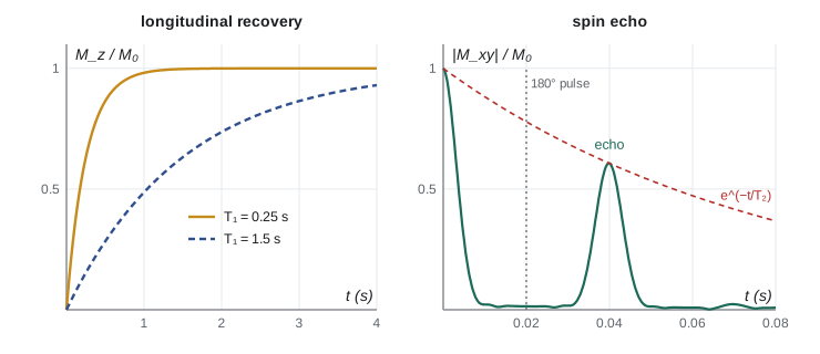
The longitudinal relaxation time \(T_1\) measures how fast the spins give energy to their surroundings and repopulate the lower level; the transverse relaxation time \(T_2\) measures how fast the precessing spins lose phase coherence with one another. In tissue both depend strongly on the molecular environment: at 1.5 T, \(T_1\) is roughly 0.25 s in fat and several seconds in cerebrospinal fluid, and \(T_2\) ranges from tens of milliseconds to over a second. These differences are the source of image contrast.

The spin echo

In a real magnet the field varies slightly from place to place, so spins in different parts of the sample precess at slightly different rates and the transverse signal fades long before \(T_2\) would require. Erwin Hahn found in 1950 how to undo this. After the \(90^\circ\) pulse, wait a time \(\tau\), during which the spins fan out in phase. Then apply a \(180^\circ\) pulse, which flips every spin across an axis in the transverse plane, reversing each one's accumulated phase. The fast spins are now behind and the slow spins ahead, and after another time \(\tau\) they all line up again: the magnetization refocuses into an echo at \(2\tau\). Inhomogeneity is undone; genuine random processes, which are what \(T_2\) measures, are not. The program simulates an ensemble of 4,000 spins with a spread of precession frequencies: the signal collapses within 10 ms, then revives at 40 ms to exactly the value \(e^{-2\tau/T_2}\) set by the true relaxation. Echoes are used in nearly every MRI sequence and in quantum computing, where the same trick, called dynamical decoupling, protects qubits from slowly varying noise.

Making images

In 1973 Paul Lauterbur realized that adding a magnetic field gradient makes the Larmor frequency depend on position, so the frequency spectrum of the signal is a projection of the spin density along the gradient. Peter Mansfield developed fast mathematical methods for reconstructing images from such data. They shared the 2003 Nobel Prize in Physiology or Medicine. A modern scanner switches gradients along three axes in microseconds, encodes position in both frequency and phase, and reconstructs each slice with a two-dimensional Fourier transform, the same mathematics as lesson 11's form factors. Choosing the timing of the pulses relative to \(T_1\) and \(T_2\) weights the image toward one or the other: \(T_1\)-weighted images show anatomy with fat bright, while \(T_2\)-weighted images make fluid and swelling bright, which is why they reveal tumors and inflammation. The superconducting magnets that produce the steady field, typically 1.5 or 3 T, are wound from niobium–titanium wire cooled by liquid helium, the boson superfluid of lesson 4 helping to image the human body.

Two spins: entanglement

For two spins one-half, the state space has four dimensions, and most of its states cannot be written as a product of a state of spin 1 and a state of spin 2. The singlet of lesson 3 is the standard example:

Such states are entangled. Neither spin alone has a definite state: measuring either one along any axis gives up or down with probability one half. Yet the outcomes are perfectly anticorrelated along every axis, and for measurements along directions \(\hat{\mathbf a}\) and \(\hat{\mathbf b}\) the average product of the results is \(E(\mathbf a, \mathbf b) = -\hat{\mathbf a}\cdot\hat{\mathbf b} = -\cos\theta_{ab}\). PHYS-372 met Bell's theorem; here is its sharpest form, the inequality of John Clauser, Michael Horne, Abner Shimony and Richard Holt (1969). Any local theory in which each particle carries predetermined answers satisfies

while quantum mechanics, for the singlet with the angles chosen in the program, gives \(2\sqrt2 = 2.83\). The program also simulates a natural local model in which each pair carries a random hidden direction; it reaches the bound of 2 and no further. Experiments since 1972, culminating in loophole-free tests in 2015 in Delft, Vienna and Boulder, find the quantum value. Entanglement is not a curiosity: it is the resource that quantum communication and computation use.

import math, random, cmath
gamma_p = 42.577478           # proton gyromagnetic ratio over 2 pi, MHz per tesla
hbar, kB = 1.054571817e-34, 1.380649e-23
print("Proton magnetic resonance")
for B in (1.5, 3.0, 7.0):
    f = gamma_p * B
    dE = 2 * math.pi * f * 1e6 * hbar
    pol = math.tanh(dE / (2 * kB * 310.0))   # net polarization at body temperature
    print(f"  B = {B:3.1f} T: Larmor {f:7.2f} MHz, spin polarization at 310 K = {pol * 1e6:5.2f} per million")
print()

# Spin echo: an ensemble of spins with spread-out precession frequencies (seeded), T2 decay included
rnd = random.Random(373)
N = 4000
offsets = [rnd.gauss(0.0, 2 * math.pi * 50.0) for _ in range(N)]   # rad/s spread (field inhomogeneity)
T2 = 0.080                                                          # s, intrinsic transverse relaxation
tau = 0.020                                                          # s, time of the 180-degree pulse
def transverse(t):
    """|<M_xy>| after a 90-degree pulse at t = 0 and a 180-degree pulse at tau."""
    s = 0j
    for d in offsets:
        phase = d * t if t < tau else d * (t - tau) - d * tau      # the 180 pulse reverses the accumulated phase
        s += cmath.exp(1j * phase)
    return abs(s) / N * math.exp(-t / T2)
print("Spin echo (90 pulse at 0, 180 pulse at 20 ms)")
for t in (0.0, 0.005, 0.010, 0.020, 0.030, 0.040, 0.050):
    print(f"  t = {t * 1000:4.0f} ms: transverse magnetization {transverse(t):.3f}   pure T2 decay {math.exp(-t / T2):.3f}")
print()

# Entanglement: CHSH correlation of the singlet, E(a, b) = -cos(a - b)
E = lambda a, b: -math.cos(a - b)
a1, a2, b1, b2 = 0.0, math.pi / 2, math.pi / 4, 3 * math.pi / 4
S = E(a1, b1) - E(a1, b2) + E(a2, b1) + E(a2, b2)
print(f"CHSH value for the singlet at the optimal angles: |S| = {abs(S):.4f}  (local limit 2, 2 sqrt 2 = {2 * math.sqrt(2):.4f})")
# a local hidden-variable model: each pair carries a random direction lam; outcomes sign(cos(angle - lam))
M = 200000
def lhv(a, b):
    tot = 0
    for _ in range(M // 4):
        lam = rnd.uniform(0, 2 * math.pi)
        A = 1 if math.cos(a - lam) >= 0 else -1
        B = -1 if math.cos(b - lam) >= 0 else 1
        tot += A * B
    return tot / (M // 4)
S_lhv = lhv(a1, b1) - lhv(a1, b2) + lhv(a2, b1) + lhv(a2, b2)
print(f"same angles with a local hidden-variable model: |S| = {abs(S_lhv):.3f}")

Proton magnetic resonance
  B = 1.5 T: Larmor   63.87 MHz, spin polarization at 310 K =  4.94 per million
  B = 3.0 T: Larmor  127.73 MHz, spin polarization at 310 K =  9.89 per million
  B = 7.0 T: Larmor  298.04 MHz, spin polarization at 310 K = 23.07 per million

Spin echo (90 pulse at 0, 180 pulse at 20 ms)
  t =    0 ms: transverse magnetization 1.000   pure T2 decay 1.000
  t =    5 ms: transverse magnetization 0.278   pure T2 decay 0.939
  t =   10 ms: transverse magnetization 0.019   pure T2 decay 0.882
  t =   20 ms: transverse magnetization 0.018   pure T2 decay 0.779
  t =   30 ms: transverse magnetization 0.015   pure T2 decay 0.687
  t =   40 ms: transverse magnetization 0.607   pure T2 decay 0.607
  t =   50 ms: transverse magnetization 0.011   pure T2 decay 0.535

CHSH value for the singlet at the optimal angles: |S| = 2.8284  (local limit 2, 2 sqrt 2 = 2.8284)
same angles with a local hidden-variable model: |S| = 1.997

Qubits

A qubit is a two-level system used to store quantum information: \(|0\rangle\) and \(|1\rangle\) play the role of a classical bit's two values, but the qubit can be in any superposition, a point on the Bloch sphere. Single-qubit gates are rotations of the Bloch vector, produced by resonant pulses exactly like those of NMR. Two-qubit gates, produced by a controlled interaction such as \(\mathbf S_1\cdot\mathbf S_2\) switched on for a set time, create entanglement. A register of \(n\) qubits has \(2^n\) basis states, and a quantum algorithm manipulates superpositions of all of them at once, using interference to make wrong answers cancel. Peter Shor showed in 1994 that a quantum computer could factor large numbers efficiently, which would break the public-key cryptography in wide use today, the reason governments standardized new post-quantum methods in 2024.

The hard part is keeping the qubits quantum. Any uncontrolled interaction with the environment acts like a measurement, destroying superpositions on a time scale analogous to \(T_2\), a process called decoherence. The leading platforms trade off coherence and control in different ways. Trapped ions, used by several groups including in Innsbruck and at NIST in Boulder, hold coherence for seconds. Superconducting qubits, small circuits of aluminum and Josephson junctions cooled to about 10 millikelvin, are fast and can be fabricated like chips; they descend directly from the experiments of John Clarke, Michel Devoret and John Martinis at Berkeley in 1984 and 1985, which showed that the current in a Josephson junction circuit has quantized energy levels and tunnels out of a metastable state as a single macroscopic quantum variable. That work earned the 2025 Nobel Prize in Physics. Canada has been prominent in the field: D-Wave in Burnaby built early superconducting quantum annealers, and the Institute for Quantum Computing in Waterloo and Xanadu in Toronto, with its photonic processors, work at the frontier; in the United States, IBM, Google and national laboratories run superconducting processors with more than a hundred qubits.

Where to go next

This course has developed the core of nonrelativistic quantum mechanics. Advanced Quantum Mechanics, PHYS-472, extends time-dependent perturbation theory and scattering, introduces density matrices for describing mixed states and decoherence, and develops entanglement and quantum information properly. Statistical Mechanics, PHYS-361, puts the Fermi and Bose distributions of lessons 4 and 5 on a thermal footing. Solid State Physics, PHYS-410, adds the crystal lattice to the free-electron gas and explains semiconductors. Nuclear and Particle Physics, PHYS-420, builds on the angular momentum coupling, the WKB treatment of alpha decay and the scattering theory developed here. Beyond those lie quantum field theory, where particles are excitations of fields, spin and statistics are explained, and the Lamb shift and the electron's \(g - 2\) are calculated to many decimal places.