Energy, potentials and stability in one dimension

Many problems in mechanics can be solved without ever finding the position as a function of time. If a force can be derived from a potential energy, conservation of energy turns the second-order equation of motion into a first-order one, and a sketch of the potential energy curve tells you at a glance where the particle can go, where it turns around, where it can rest, and whether a small push makes it return or run away. This lesson develops these energy methods for motion in one dimension and finishes with an exact formula for the period of any one-dimensional oscillation, which we use to find how a pendulum's period grows with amplitude.

Work, kinetic energy and conservative forces

Multiply Newton's second law \(m\ddot x = F\) by \(\dot x\). The left side is \(\frac{d}{dt}\big(\tfrac12m\dot x^2\big)\), so integrating between two times gives the work–energy theorem: the change in kinetic energy equals the work \(W = \int F\,dx\) done by the net force. This is true for any force. A force is called conservative if the work it does between two points depends only on the points and not on the path or on how fast the particle travels between them. In one dimension, any force that depends only on position is conservative, and we can define a potential energy

The reference point \(x_0\), where \(U = 0\), is arbitrary; only differences in \(U\) have physical meaning. With \(F = -U'\), the work–energy theorem becomes the conservation of mechanical energy,

Forces that depend on velocity (drag, friction) or explicitly on time (a driving force) are not conservative in this sense. Friction converts mechanical energy into heat; a time-dependent force can pump energy in or out. In three dimensions there is an extra condition, which lesson 6 develops: a position-dependent force is conservative only if its curl is zero.

Reading a potential energy curve

Because kinetic energy can never be negative, the particle can only be where \(U(x) \le E\). Draw a horizontal line at height \(E\) across the graph of \(U(x)\). The particle is confined to the regions where the curve lies below the line. Where the line meets the curve, \(\dot x = 0\): these are turning points, where the particle stops momentarily and reverses. Between two turning points the motion is a back-and-forth oscillation. If the region is bounded on only one side, the particle comes in, turns around and leaves for good.

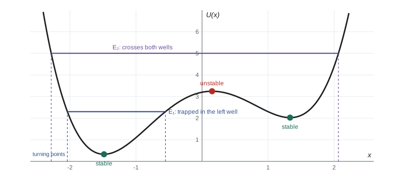
The speed at any point follows directly: \(|\dot x| = \sqrt{2(E - U(x))/m}\). The particle moves fastest where the potential is lowest. Points where \(U'(x) = 0\) are equilibria, since the force vanishes there. At a minimum of \(U\), a small displacement produces a force back toward the equilibrium, so the equilibrium is stable. At a maximum, a small displacement produces a force away from it, so the equilibrium is unstable. A double well like the one in the figure models a molecule that can sit in two configurations, a buckled beam that can snap between two shapes, or a ball on a dented surface.

Small oscillations about a minimum

Expand the potential about a stable equilibrium \(x_0\) in a Taylor series: \(U(x) = U(x_0) + \tfrac12U''(x_0)(x - x_0)^2 + \tfrac16U'''(x_0)(x - x_0)^3 + \cdots\). The linear term is absent because \(U'(x_0) = 0\). For small displacements the quadratic term dominates, and the force is \(F \approx -U''(x_0)(x - x_0)\), a spring with stiffness \(k = U''(x_0)\). The motion is simple harmonic with

This is why simple harmonic motion is everywhere, as PHYS-230 lesson 1 emphasized: almost any system near a stable equilibrium oscillates harmonically for small enough amplitude. If \(U''(x_0) < 0\) the equilibrium is unstable, and a displacement grows as \(e^{\lambda t}\) with \(\lambda = \sqrt{-U''(x_0)/m}\). If \(U''(x_0) = 0\) the quadratic test is inconclusive, and higher derivatives decide; the quartic well \(U = cx^4\) is stable, but its oscillations are not harmonic at any amplitude.

The period as an integral

Energy conservation gives the speed at each point, and the time to travel a distance \(dx\) is \(dx/|\dot x|\). Adding up the time between the turning points \(x_1\) and \(x_2\) and doubling for the return trip,

This formula holds for any one-dimensional potential well, harmonic or not. For \(U = \tfrac12kx^2\) the integral is \(\pi\sqrt{2/k}\), giving \(T = 2\pi\sqrt{m/k}\) independent of amplitude, the defining property of the harmonic oscillator. For any other well the period depends on the energy. The integrand blows up at the turning points, where the particle is momentarily at rest, but the singularity is integrable: near a turning point \(E - U \propto |x - x_i|\), and \(\int dx/\sqrt{x}\) is finite. Numerically, the substitution \(x = x_m\sin\phi\) for a symmetric well removes the singularity entirely.

The exact period of a pendulum

For a pendulum of length \(\ell\) the angle \(\theta\) plays the role of \(x\), the moment of inertia \(m\ell^2\) plays the role of \(m\), and \(U = mg\ell(1 - \cos\theta)\). Released from rest at \(\theta_0\), energy conservation gives \(\dot\theta^2 = (2g/\ell)(\cos\theta - \cos\theta_0)\). The period integral becomes

where \(K(k) = \int_0^{\pi/2}d\phi/\sqrt{1 - k^2\sin^2\phi}\) is the complete elliptic integral of the first kind, reached by the substitution \(\sin(\theta/2) = \sin(\theta_0/2)\sin\phi\). Carl Friedrich Gauss discovered in 1799 that \(K\) can be computed with astonishing speed using the arithmetic–geometric mean: \(K(k) = \pi/\big(2\,\mathrm{AGM}(1, \sqrt{1 - k^2})\big)\). Each AGM iteration roughly doubles the number of correct digits. For the pendulum, \(\sqrt{1 - k^2} = \cos(\theta_0/2)\), so

The program evaluates the period both by numerical integration of the general formula and by the AGM, for amplitudes from \(10^\circ\) to \(179^\circ\), and then applies the same integral to a quartic well.

import math

# Period of oscillation in a potential U(x) at energy E: T = 2 * integral of dx / v between turning points.
# The substitution x = xm sin(phi) removes the square-root singularity at the turning points (for even U).
def period(U, m, xm, n=2000):
    E = U(xm)
    total = 0.0
    for i in range(n):                                   # midpoint rule in phi
        phi = (i + 0.5) * (math.pi / 2) / n
        x = xm * math.sin(phi)
        v = math.sqrt(2 * (E - U(x)) / m)
        total += xm * math.cos(phi) / v * (math.pi / 2) / n
    return 4 * total

def agm(a, b):
    while abs(a - b) > 1e-15 * a:
        a, b = (a + b) / 2, math.sqrt(a * b)
    return a

g, L = 9.81, 1.0
T0 = 2 * math.pi * math.sqrt(L / g)
U_pend = lambda th: (g / L) * (1 - math.cos(th))        # per unit m L^2
print(" amplitude   T/T0 (integral)   T/T0 (AGM)")
for deg in (10, 30, 60, 90, 120, 150, 170, 179):
    th0 = math.radians(deg)
    T_int = period(U_pend, 1.0, th0)
    T_agm = 2 * math.pi / agm(1.0, math.cos(th0 / 2)) * math.sqrt(L / g)
    print(f"   {deg:3d} deg      {T_int / T0:9.5f}       {T_agm / T0:9.5f}")

# A quartic well U = c x^4: the period depends on amplitude as 1/A
c = 1.0
for A in (0.5, 1.0, 2.0):
    print(f"quartic well, A = {A}: T = {period(lambda x: c * x ** 4, 1.0, A):.4f}")

 amplitude   T/T0 (integral)   T/T0 (AGM)
    10 deg        1.00191         1.00191
    30 deg        1.01741         1.01741
    60 deg        1.07318         1.07318
    90 deg        1.18034         1.18034
   120 deg        1.37288         1.37288
   150 deg        1.76220         1.76220
   170 deg        2.43936         2.43936
   179 deg        3.90107         3.90107
quartic well, A = 0.5: T = 7.4163
quartic well, A = 1.0: T = 3.7081
quartic well, A = 2.0: T = 1.8541

The two methods agree to five decimal places at every amplitude. At \(10^\circ\) the period is only 0.19% longer than the small-angle value, which is why pendulum clocks with small swings keep good time. At \(90^\circ\) it is 18% longer, and as the amplitude approaches \(180^\circ\) the period grows without limit: at \(179^\circ\) it is almost four times the small-angle period. A pendulum released exactly upside down would balance forever at the unstable equilibrium. Near that point the time spent creeping away from the top grows logarithmically as the starting angle approaches \(180^\circ\), which is why the last few degrees add so much.

The quartic well shows the opposite trend: doubling the amplitude halves the period. Dimensional analysis predicts this. With \(U = cx^4\), the only time that can be formed from \(m\), \(c\) and the amplitude \(A\) is \(\sqrt{m/c}/A\), so \(T \propto 1/A\). In a well that stiffens faster than a spring, larger oscillations are quicker; in one that softens, like the pendulum, they are slower. Lesson 5 shows how these amplitude-dependent frequencies change the response of a driven oscillator.

Unbounded motion and escape

When the energy line lies above the potential on one side all the way to infinity, the particle escapes in that direction. For a particle launched straight up from a planet of mass \(M\) and radius \(R\), \(U(r) = -GMm/r\) rises toward zero at infinity. The particle escapes if \(E \ge 0\), that is if \(\tfrac12mv^2 \ge GMm/R\), giving the escape speed \(v_{\text{esc}} = \sqrt{2GM/R}\): 11.2 km/s from the Earth, 2.4 km/s from the Moon, 5.0 km/s from Mars. The time to travel any distance in unbounded motion follows from the same integral \(\int dx/|\dot x|\) without the factor of two.

Phase portraits from the potential

The energy equation also draws the phase portrait, the family of curves in the \((x, \dot x)\) plane traced by the motion, without solving anything: each curve is \(\dot x = \pm\sqrt{2(E - U)/m}\). Near a minimum the curves are small closed ellipses, as for the harmonic oscillator. Near a maximum they form a cross, with two branches leading in and two leading out. The curve that passes through an unstable equilibrium is the separatrix. It divides motions of different kinds, such as the back-and-forth swing of a pendulum and its continuous rotation over the top, as the phase portraits in PHYS-230 lesson 2 showed. In lesson 12 we will see that driving or coupling can shatter the separatrix into a tangle of chaotic motion.