Why classical mechanics: from Newton to the edge of chaos

Classical mechanics is the physics of how things move when they are much larger than atoms and much slower than light. It predicts the path of a thrown ball, the orbit of a satellite, the wobble of a spinning top and the swing of a bridge in the wind. It is also the oldest mathematical science still in daily use, and the place where most of the ideas of modern physics were first worked out: conservation laws, the link between symmetry and conservation, the description of motion in a space of states, and the discovery that perfectly deterministic equations can still produce behavior that cannot be predicted in practice. This course takes the mechanics you met in PHYS-130 and develops it into the tool that working physicists and engineers actually use.

PHYS-130 introduced Newton's laws, energy, momentum, rotation, gravitation and simple oscillations, mostly in one or two dimensions and mostly with constant forces. Here the forces vary with position, velocity and time, the motion is often three-dimensional, and the reference frames rotate. We will solve the equations exactly where we can and numerically where we cannot, and in every lesson a short Python program checks the mathematics. PHYS-230 treated linear oscillations, damping, resonance and coupled oscillators in depth; we build on that work in lesson 5 rather than repeat it, and move on to oscillators whose restoring force is not linear. The sequel, PHYS-344, reformulates everything in this course in the language of Lagrange and Hamilton.

The program of this course

The course has four parts. Lessons 1 to 6 sharpen the foundations: Newton's laws for systems of particles, motion with drag and with changing mass, energy methods in one dimension, nonlinear oscillators, and the vector calculus needed in three dimensions. Lessons 7 to 9 treat motion under central forces, the problem that launched the whole subject: the two-body problem, Kepler's laws, orbital maneuvers and the scattering of one particle by another. Lessons 10 and 11 deal with rotation, first of the reference frame (centrifugal and Coriolis effects, the Foucault pendulum) and then of the body itself (the inertia tensor, Euler's equations and gyroscopes). Lesson 12 closes with chaos, where we find that Newton's deterministic laws can generate motion that is, for all practical purposes, unpredictable.

A short history

Galileo's Two New Sciences of 1638 established that falling bodies accelerate uniformly and that a projectile's horizontal and vertical motions are independent. Johannes Kepler, working from Tycho Brahe's naked-eye observations of Mars, published his first two laws of planetary motion in Astronomia Nova in 1609 and the third, relating period to orbit size, in Harmonices Mundi in 1619. Isaac Newton's Principia of 1687 unified the two: the same law of gravitation that pulls an apple to the ground holds the Moon and planets in their orbits, and Kepler's three laws follow from it as theorems. We prove them in lessons 7 and 8.

The eighteenth century turned Newton's geometric arguments into calculus. Leonhard Euler wrote mechanics as differential equations, worked out the motion of rigid bodies in his Theoria motus corporum solidorum of 1765, and introduced much of the notation we still use. Joseph-Louis Lagrange's Mécanique analytique of 1788 removed geometry altogether, and William Rowan Hamilton in the 1830s gave the theory the form that later carried over into quantum mechanics. At the end of the nineteenth century Henri Poincaré, studying the three-body problem for a prize offered by King Oscar II of Sweden, found that some orbits are so tangled that no simple formula can describe them. That discovery, largely ignored for seventy years, re-emerged in the 1960s as the theory of chaos.

Newton's laws as differential equations

The central idea of the course is that Newton's second law is a differential equation. For a particle of mass \(m\) acted on by a total force \(\mathbf F\) that may depend on position, velocity and time,

This is a second-order equation for the vector \(\mathbf r(t)\). Given the position and velocity at one instant, the theory of differential equations guarantees (for any reasonably smooth force) a unique solution for all later times. That is the precise meaning of determinism in classical mechanics: the present state fixes the future. Pierre-Simon Laplace expressed it in 1814 with his imagined intellect that, knowing every position and velocity, could compute the whole future of the universe.

It is convenient to write the second-order equation as a first-order system. Define the state as the pair \((\mathbf r, \mathbf v)\); then

For a particle in three dimensions the state has six numbers, and the motion traces a curve through a six-dimensional state space. For \(N\) particles the state space has \(6N\) dimensions. This picture, which you met for a single oscillator in PHYS-230, is how both the numerical methods of this course and the theory of chaos in lesson 12 think about motion: as the flow of a point through a space of states.

Where classical mechanics applies

Newton's laws are an approximation, and an excellent one in a wide domain. They fail in two directions. When speeds approach the speed of light \(c\), special relativity takes over; the size of the correction is set by \(v/c\), and effects scale as \((v/c)^2\). When the de Broglie wavelength \(\lambda = h/p\) of an object becomes comparable to the size of the region it moves in, quantum mechanics takes over. A third limit, very strong gravity, belongs to general relativity, the subject of PHYS-450.

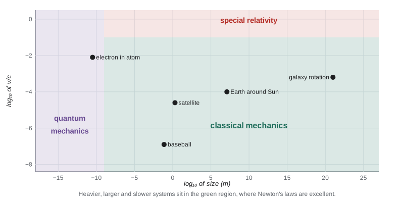
These criteria are easy to evaluate, and the program below does so for a range of systems. It also introduces the fourth-order Runge–Kutta method, RK4, that we will use throughout the course to integrate equations of motion that have no closed-form solution.

import math

# Where does classical mechanics apply? Compare speed with c and size with the de Broglie wavelength.
h, c = 6.626e-34, 2.998e8
cases = [  # name, mass (kg), speed (m/s), size (m)
    ("baseball pitch", 0.145, 40.0, 0.074),
    ("satellite in low orbit", 1000.0, 7.7e3, 2.0),
    ("dust grain in air", 1e-15, 0.01, 1e-6),
    ("electron in a TV-style tube", 9.11e-31, 6e7, 1e-3),
    ("electron in an atom", 9.11e-31, 2.2e6, 1e-10),
    ("proton at the LHC", 1.67e-27, 0.999999990 * c, 1e-15),
]
print(f"{'system':28s} {'v/c':>9s} {'lambda/size':>12s}  verdict")
for name, m, v, L in cases:
    beta = v / c
    gamma = 1 / math.sqrt(1 - beta * beta)
    lam = h / (gamma * m * v)
    rel, quant = beta > 0.1, lam / L > 0.01
    verdict = "classical" if not (rel or quant) else ("relativistic " if rel else "") + ("quantum" if quant else "")
    print(f"{name:28s} {beta:9.2e} {lam / L:12.2e}  {verdict.strip()}")

# A general-purpose RK4 step, used throughout the course, tested on free fall
def rk4(f, t, y, dt):
    k1 = f(t, y)
    k2 = f(t + dt / 2, [a + dt / 2 * b for a, b in zip(y, k1)])
    k3 = f(t + dt / 2, [a + dt / 2 * b for a, b in zip(y, k2)])
    k4 = f(t + dt, [a + dt * b for a, b in zip(y, k3)])
    return [a + dt / 6 * (b1 + 2 * b2 + 2 * b3 + b4) for a, b1, b2, b3, b4 in zip(y, k1, k2, k3, k4)]

g = 9.81
fall = lambda t, y: [y[1], -g]          # state (height, velocity)
for dt in (0.1, 0.01):
    t, y = 0.0, [100.0, 0.0]
    while t < 3.0 - 1e-12:
        y = rk4(fall, t, y, dt); t += dt
    print(f"dt = {dt}: height after 3 s = {y[0]:.10f} m (exact {100 - 0.5 * g * 9:.10f})")

system                             v/c  lambda/size  verdict
baseball pitch                1.33e-07     1.54e-33  classical
satellite in low orbit        2.57e-05     4.30e-41  classical
dust grain in air             3.34e-11     6.63e-11  classical
electron in a TV-style tube   2.00e-01     1.19e-08  relativistic
electron in an atom           7.34e-03     3.31e+00  quantum
proton at the LHC             1.00e+00     1.87e-04  relativistic
dt = 0.1: height after 3 s = 55.8550000000 m (exact 55.8550000000)
dt = 0.01: height after 3 s = 55.8550000000 m (exact 55.8550000000)

The baseball and the satellite are classical by an enormous margin: their de Broglie wavelengths are around \(10^{-33}\) and \(10^{-41}\) times their size. An electron in an atom has a wavelength larger than the atom, so its motion must be treated quantum mechanically. The electron in an old television tube is moving at about a fifth of light speed, so relativistic corrections of around 2% matter for a precise design. A proton at the Large Hadron Collider is extremely relativistic. The RK4 integrator reproduces free fall exactly, to every printed digit, because RK4 integrates polynomials of degree up to four without error; for the forces of later lessons it is accurate to a relative error proportional to \(\Delta t^4\).

How RK4 works

The simplest way to step a first-order system \(\dot y = f(t, y)\) forward is Euler's method, \(y_{n+1} = y_n + \Delta t\, f(t_n, y_n)\). It uses the slope only at the start of the step, so its error per step is proportional to \(\Delta t^2\) and its accumulated error over a fixed time is proportional to \(\Delta t\). Halving the step only halves the error. The fourth-order Runge–Kutta method, published by Carl Runge in 1895 and extended by Wilhelm Kutta in 1901, samples the slope four times per step:

The weights are chosen so that the result agrees with the Taylor series of the exact solution through the \(\Delta t^4\) term. The accumulated error is then proportional to \(\Delta t^4\): halving the step reduces it sixteenfold. RK4 does not conserve energy exactly, and over very long runs its energy drifts slowly. For orbits followed over thousands of periods we will switch, as PHYS-230 did for oscillators, to the velocity Verlet method, which keeps the energy error bounded.

Dimensional analysis

Before solving any problem it pays to ask which combinations of the given quantities have the right dimensions. A simple pendulum has length \(\ell\), mass \(m\) and swings in a gravitational field \(g\). The only combination with the dimension of time is \(\sqrt{\ell/g}\); the mass cannot enter, because no other quantity contains kilograms to cancel it. So the period must be \(T = C\sqrt{\ell/g}\) with a dimensionless constant \(C\), which for small swings turns out to be \(2\pi\). The amplitude \(\theta_0\) is itself dimensionless, so in general \(C\) can depend on it; lesson 4 computes that dependence exactly.

The general statement, the Buckingham pi theorem of 1914, says that a relation among \(n\) quantities involving \(k\) independent units can be rewritten as a relation among \(n - k\) dimensionless groups. The pendulum has four quantities \((T, \ell, g, \theta_0)\) and two units (length and time), giving two groups, \(T\sqrt{g/\ell}\) and \(\theta_0\). Dimensional analysis cannot find the constant, but it tells you what the answer can depend on and how it scales, which is often the most useful thing to know.

Conservation laws as tools

Three quantities are conserved in an isolated system: momentum, angular momentum and energy. In lesson 2 we derive each from Newton's laws. They matter because they reduce the work of solving the equations. A particle in three dimensions needs six numbers to specify its state. If energy and the three components of angular momentum are conserved, four combinations of those six numbers stay fixed, and the motion is confined to a two-dimensional surface in state space. Kepler's problem in lesson 7 is solved exactly this way.

Conservation laws come from symmetries. Momentum is conserved because the laws of physics are the same everywhere, angular momentum because they are the same in every direction, and energy because they do not change with time. This connection, proved in general by Emmy Noether in 1918, is developed in PHYS-344. In this course we will see it case by case: a force that depends only on the distance from a center is symmetric under rotation, and the angular momentum about that center is conserved.

Predictability and its limits

Determinism and predictability are not the same. Determinism says that the exact present state fixes the future. Predictability requires that a slightly uncertain present state fixes the future to within a slightly uncertain range. For a pendulum swinging gently, or a planet in a simple orbit, small errors in the starting conditions grow slowly, roughly in proportion to time, and long-range prediction works. For a double pendulum swinging wildly, the errors grow exponentially, doubling every fraction of a second, and no measurement could be precise enough to predict its position a minute ahead. Both systems obey Newton's laws exactly. Lesson 12 explains how to tell which kind of system you have and how to measure the rate at which predictability is lost.

Edward Lorenz found this behavior in 1963 in a simplified model of atmospheric convection, and his observation is the reason weather forecasts lose skill after a week or two however powerful the computer. Chaos does not mean that physics fails; it means that some questions (exactly where will the pendulum be in an hour?) must be replaced by statistical ones (how much of the time does it spend in each region?). Even the solar system, the model of clockwork regularity, turns out to be chaotic on time scales of millions of years.