
PET-420 · Lesson 9 of 12 · 19 min
Two-phase flow, numerical dispersion and grid effects
The pilot's first producer saw water about eleven months after injection began, earlier than the analytical waterflood estimate in the original pilot design. Before trusting the simulator to explain why, Lena wants Ethan to know how the simulator itself moves a waterfront, and how the numerical method can make a front arrive too early or too late regardless of the geology. 'A simulator does not solve Buckley-Leverett,' she says. 'It solves something close to it on a grid, and the difference depends on your block size. You need to know how big the difference is before you blame the rock.'
The saturation equation
For one-dimensional incompressible flow of oil and water without gravity or capillary pressure, the water mass balance and Darcy's law reduce to a single equation for water saturation, the Buckley-Leverett equation:
The fractional flow f_w is the fraction of the total flow that is water, and depends on saturation through the relative permeabilities and on the viscosity ratio. The equation is hyperbolic: saturations travel at speeds proportional to df_w/dS_w, so a given saturation moves along the flood at a constant speed. Because the speed is greatest at intermediate saturations, the faster saturations would overtake the slower ones, and the physically correct solution contains a shock, a sharp front at which the water saturation jumps from its connate value to the front saturation. Welge's tangent construction finds the front saturation as the point where a line from the connate saturation touches the fractional flow curve. The front reaches the producer, and water breaks through, when the injected volume in pore volumes equals the inverse of the slope at the front.
Upstream weighting
In a simulator, the saturation equation is discretized like the pressure equation, with one important difference. The mobility used for flow across each face must be evaluated somewhere, and the choice decides whether the scheme behaves. Using the average of the two blocks seems natural, but for a hyperbolic equation it produces oscillations and non-physical saturations. The standard choice is single-point upstream weighting: the mobility of each phase across a face is taken from the block on the upstream side, the side from which that phase is flowing.
Upstream weighting has a clear physical meaning. Water cannot flow into a block at the mobility of water in that block if the block contains no water; it flows at the mobility it has in the block it is coming from. The scheme is stable, gives physically bounded saturations and handles fronts reliably. Its cost is accuracy. It is only first-order accurate in space, and it introduces an error that behaves exactly like a diffusion term.
Numerical dispersion
A Taylor series analysis of the upstream scheme shows that it solves not the Buckley-Leverett equation but one with an extra term of the form D_num ∂²S_w/∂x², with an artificial diffusion coefficient proportional to the block size and the wave speed:
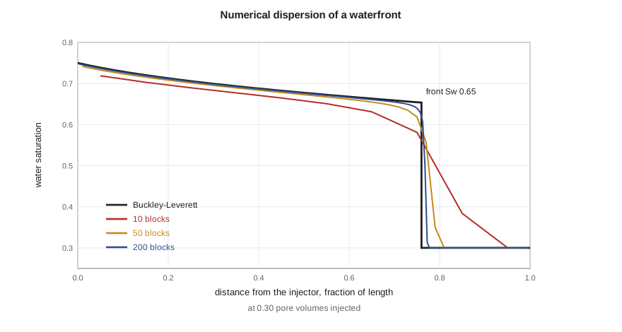
where v is the saturation wave speed. This numerical dispersion smears the sharp Buckley-Leverett front over several blocks. The leading edge of the smeared front, carrying small water saturations, runs ahead of the true front and reaches the producer early. Breakthrough in a coarse model therefore occurs too soon and water cut rises too gradually, while oil recovery at a given injected volume is slightly understated before breakthrough and the post-breakthrough performance is blurred.
The code below solves the one-dimensional waterflood with upstream weighting on grids of 10, 50 and 200 blocks and compares each with the Buckley-Leverett solution for the Mission Canyon pool relative permeabilities and an oil viscosity of 0.95 cp.
# 1D waterflood: IMPES-style upstream-weighted saturation update versus the Buckley-Leverett solution
SI = False
if SI: swc, sor, muo, muw, no, nw, kro0, krw0 = 0.30, 0.25, 0.72, 0.45, 2.0, 2.5, 0.85, 0.30
else:  swc, sor, muo, muw, no, nw, kro0, krw0 = 0.30, 0.25, 0.95, 0.45, 2.0, 2.5, 0.85, 0.30
def fw(s):                                   # fractional flow of water (no gravity, no capillary pressure)
    se = min(max((s - swc) / (1 - swc - sor), 0.0), 1.0)
    lw = krw0 * se ** nw / muw; lo = kro0 * (1 - se) ** no / muo
    return lw / (lw + lo)
def dfw(s, h=1e-6): return (fw(s + h) - fw(s - h)) / (2 * h)
# Welge tangent: front saturation where fw(s)/(s - swc) = dfw/ds
best = max((fw(s) / (s - swc), s) for s in [swc + 0.0005 * i for i in range(1, 900)] if s < 1 - sor)
sf = best[1]; bt = 1 / dfw(sf)
print(f"Buckley-Leverett: front Sw = {sf:.3f}, breakthrough at {bt:.3f} pore volumes injected")
def simulate(n, pv_end=1.0, cfl=0.4):
    s = [swc] * n; dx = 1.0 / n; t = 0.0; bt_pv = None
    vmax = max(dfw(swc + 0.01 * i) for i in range(1, 45))
    dt = cfl * dx / vmax
    while t < pv_end:
        f = [fw(x) for x in s]
        new = s[:]
        new[0] = s[0] + dt / dx * (1.0 - f[0])          # injector face carries water only
        for i in range(1, n): new[i] = s[i] + dt / dx * (f[i - 1] - f[i])
        s = new; t += dt
        if bt_pv is None and fw(s[-1]) > 0.01: bt_pv = t
    return s, bt_pv
for n in (10, 50, 200):
    s, b = simulate(n, 0.30)
    front = sum(1 for x in s if x > swc + 0.02) / n
print(f"{n:3d} blocks: water reached {front:.2f} of the length at 0.30 PV (exact {0.30 * dfw(sf):.2f}); breakthrough at {simulate(n, 0.8)[1]:.3f} PV")Buckley-Leverett: front Sw = 0.653, breakthrough at 0.395 pore volumes injected 10 blocks: water reached 0.90 of the length at 0.30 PV (exact 0.76); breakthrough at 0.342 PV 50 blocks: water reached 0.80 of the length at 0.30 PV (exact 0.76); breakthrough at 0.380 PV 200 blocks: water reached 0.77 of the length at 0.30 PV (exact 0.76); breakthrough at 0.390 PV
The analytical solution gives a front saturation of about 0.65 and breakthrough at about 0.40 pore volumes injected. With 10 blocks the leading edge of the water has already reached 90 percent of the length when the true front is at about three quarters, and breakthrough comes at about 0.34 pore volumes, some 13 percent early. With 50 blocks the error is a few percent, and with 200 blocks the numerical solution is close to the analytical one. Lena's pilot model has about eight blocks between injector and producer in each direction, so it is closer to the coarse case than the fine one. Part of the early breakthrough the model will show is numerical, and that has to be accounted for before the thief layer is blamed for all of it.
Reducing numerical dispersion
Several remedies are available. Refining the grid is the simplest and the most expensive; because the error scales with block size, halving the blocks roughly halves the smearing but multiplies the cost by four in two dimensions and eight in three, before accounting for shorter time steps. Higher-order schemes, such as flux-limited or total variation diminishing methods, keep fronts sharp without oscillations by using second-order accuracy away from fronts and falling back to upstream weighting near them; they are used in some compositional and research codes. Front-tracking and streamline methods move saturations along streamlines with one-dimensional solutions that have little numerical dispersion; streamline simulators are popular for fast screening of large waterflood models.
Pseudo-relative permeabilities, mentioned in Lesson 7, can also compensate for numerical dispersion: a coarse-grid curve is tuned so that the coarse model reproduces a fine-grid or analytical breakthrough time. This is effective when the flow conditions are well defined, but it mixes a numerical correction with a physical property and can confuse the history match later. Lena prefers to quantify the numerical error with a fine-grid cross-section and to keep it in mind when interpreting the match.
Mobility ratio, fingering and grid orientation
The end-point mobility ratio M, the mobility of water at residual oil divided by the mobility of oil at connate water, decides whether a displacement is stable. When M is less than one, the displacing water is less mobile than the oil it pushes and any irregularity in the front tends to heal. When M is well above one, small perturbations grow into viscous fingers that bypass oil. Grids cannot resolve fingers that are smaller than a block, and coarse models of unfavorable floods tend to overstate sweep. The pilot's end-point mobility ratio is below one, so fingering is not the main concern, but the thief layer gives the same effect on a larger scale.
In two and three dimensions, numerical dispersion also depends on the direction of flow relative to the grid. On a Cartesian grid with five-point connections, a front moving along the grid axes behaves differently from one moving diagonally, so a five-spot pattern simulated with the producer diagonal to the injector gives a different breakthrough time from the same pattern rotated 45 degrees. This grid orientation effect is strongest for unfavorable mobility ratios. Nine-point schemes, which add diagonal connections, reduce it, as do grids aligned with the main flow directions.
Gravity and capillary pressure
Real displacements also feel gravity and capillary pressure. Water is denser than oil, so in thick or high-permeability layers it tends to slump toward the base, a process called gravity underride, while injected gas tends to override toward the top. The ratio of viscous to gravity forces decides how strongly this happens and is often expressed as a viscous-gravity number. Capillary pressure opposes the sharpening of fronts and spreads them over a capillary transition length, which is physical dispersion rather than numerical. In fine-scale models of heterogeneous rock, capillary pressure also causes water to imbibe from high-permeability layers into tighter neighbors, a crossflow that can improve the sweep of layered reservoirs. Coarse models with averaged properties cannot represent it unless the layers are kept separate.
| Effect | Cause | Result in a simulation | Remedy |
|---|---|---|---|
| Numerical dispersion | First-order upstream weighting | Smeared fronts, early breakthrough | Finer grid, higher-order or streamline methods |
| Grid orientation | Five-point connections | Breakthrough depends on grid direction | Nine-point schemes, aligned grids |
| Viscous fingering | Unfavorable mobility ratio | Unresolved, sweep overstated on coarse grids | Fine grids, pseudo-functions |
| Gravity segregation | Density difference | Underride or override in thick layers | Enough vertical resolution |
| Capillary dispersion | Capillary pressure gradients | Physical smearing and crossflow | Keep layers separate with correct curves |
Worked problem
How early is a coarse-grid breakthrough?
The analytical breakthrough of a linear flood is at 0.40 pore volumes injected. A ten-block simulation breaks through at 0.35 pore volumes. If the pilot injects 1,040 bbl/d into a pattern pore volume of 2.64 million bbl, how many days early does the coarse model predict breakthrough?
Show solution
- The analytical breakthrough occurs after 0.40 × 2.64 million = 1.056 million bbl injected, or 1,056,000 / 1,040 = 1,015 days.
- The coarse model breaks through after 0.35 pore volumes, 924,000 bbl or about 888 days.
- The difference is about 127 days, or roughly four months.
Answer: The coarse model predicts breakthrough about four months early on numerical grounds alone. The engineer must account for this before attributing the difference to geology.
A fine cross-section for the pilot
To measure the numerical error in the pilot model, Ethan builds a two-dimensional vertical cross-section from the injector to the first producer with the same layering but blocks only 16 ft long, ten times finer than the full model. He runs it with the same properties and compares it with the corresponding row of the coarse model. The coarse row breaks through about two months earlier than the fine cross-section, and its water cut rises more gradually. The difference is smaller than in the one-dimensional example because the thief layer dominates both runs: once the water is in the streak, it reaches the producer quickly on either grid. Lena records the comparison in the study report as an estimate of the numerical part of the breakthrough timing, so that the history match does not try to remove it with changes to the geology.
Common mistakes
MistakeUsing central weighting of mobility for saturation transport.
InsteadUse upstream weighting, which is stable and keeps saturations physical.
MistakeBlaming early simulated breakthrough entirely on geology.
InsteadQuantify numerical dispersion first, for example with a fine-grid cross-section.
MistakeAssuming a coarse grid is conservative for sweep.
InsteadCoarse grids can either overstate or understate sweep; fingers and streaks may be unresolved.
MistakeIgnoring the grid direction in pattern floods.
InsteadCheck grid orientation effects, especially for unfavorable mobility ratios.
Summary and key terms
- The saturation equation is hyperbolic, and its exact solution for a waterflood contains a shock front found by Welge's tangent.
- Simulators use single-point upstream weighting of mobilities, which is stable but first-order accurate.
- Upstream weighting adds numerical dispersion proportional to block size, smearing fronts and causing early breakthrough.
- Finer grids, higher-order schemes and streamline methods reduce numerical dispersion.
- Mobility ratio controls fingering; five-point grids add orientation effects for unfavorable floods.
- Gravity and capillary pressure are physical effects that the grid must resolve vertically to represent.
- Fractional flow
- The fraction of the total flow that is water, as a function of saturation.
- Shock front
- A sharp jump in saturation that travels at constant speed in a Buckley-Leverett displacement.
- Upstream weighting
- Evaluating the mobility across a face from the block on the upstream side of the flow.
- Numerical dispersion
- Artificial smearing of fronts caused by the truncation error of the numerical scheme.
- Mobility ratio
- The mobility of the displacing phase divided by that of the displaced phase.
- Grid orientation effect
- Dependence of simulated results on the direction of flow relative to the grid axes.
- Streamline simulation
- A method that solves saturation transport along streamlines computed from the pressure field.
Practice problems
Work each problem on paper first, then reveal the answer to check.
Why is upstream weighting physically sensible?
Show answer
A phase flows into a block at the mobility it has in the block it is coming from.
Why does numerical dispersion cause early breakthrough?
Show answer
The smeared front's leading edge, carrying small water saturations, runs ahead of the true front.
How does numerical dispersion scale with block size?
Show answer
Roughly in proportion to the block size, so finer blocks reduce it.
When is the grid orientation effect strongest?
Show answer
For unfavorable mobility ratios on five-point Cartesian grids.
Lesson quiz · 5 questions
Score 60% or more to complete this lesson.
Create a free account to save your progress, take quizzes and earn a certificate.