
PET-420 · Lesson 12 of 12 · 19 min
Capstone: simulating the waterflood pilot
Eight months after Ethan joined the simulation work, the study is ready to present. The pilot-area model reproduces the pool pressure, the breakthrough at the first producer and the water cuts at the other three. An ensemble of matched models carries the remaining uncertainty into the forecasts. This capstone lesson pulls the course together in two parts. The first is a small two-dimensional simulator that Ethan writes himself, a quarter of a five-spot pattern, to see every piece of the method working at once. The second is the study itself: how the model was built and matched, what it predicts and what Lena and Ethan recommend for the Mission Canyon pool.
A pattern simulator from first principles
The five-spot is the classic waterflood pattern: an injector at the center of a square with a producer at each corner, or equivalently a producer at the center of a square of injectors. By symmetry, one quarter of the pattern, a square with an injector at one corner and a producer at the opposite corner, behaves like the whole. Ethan's program grids that quarter into 15 by 15 blocks of equal size, with uniform permeability and the pool's relative permeability curves, and simulates incompressible oil-water flow with the IMPES method of Lesson 4.
Each part of the program corresponds to a lesson. The pressure equation is the finite-volume balance of Lesson 3 in two dimensions, with harmonic averages of the total mobility at each face, solved by successive over-relaxation, a simple iterative solver of the kind described in Lesson 5. The injector and producer are source and sink terms in their corner blocks, with the producer held at a reference pressure. The saturation update is explicit, with upstream-weighted fractional flows as in Lesson 9, and the time step is kept small enough to satisfy the throughput limit. Pressure is recomputed every few saturation steps, because the total mobility changes slowly compared with the saturations.
# Capstone: quarter five-spot waterflood on a 2D grid (incompressible, IMPES, upstream weighting)
SI = False
nx = ny = 15
if SI: swc, sor, muo, muw, krw0, kro0 = 0.30, 0.25, 0.72, 0.45, 0.30, 0.85
else:  swc, sor, muo, muw, krw0, kro0 = 0.30, 0.25, 0.95, 0.45, 0.30, 0.85
def mob(s):
    se = min(max((s - swc) / (1 - swc - sor), 0.0), 1.0)
    return krw0 * se ** 2.5 / muw, kro0 * (1 - se) ** 2 / muo
S = [ [swc] * nx for _ in range(ny)]
pv_cell = 1.0 / (nx * ny); q = 1.0                     # inject 1 pore volume per unit time at cell (0,0)
def pressure(S):
    lam = [ [sum(mob(S[j][i])) for i in range(nx)] for j in range(ny)]
    P = [ [0.0] * nx for _ in range(ny)]
    for _ in range(600):                                # successive over-relaxation
        for j in range(ny):
            for i in range(nx):
                if (i, j) == (nx - 1, ny - 1): P[j][i] = 0.0; continue
                num = q if (i, j) == (0, 0) else 0.0; den = 0.0
                for a, b in ((i - 1, j), (i + 1, j), (i, j - 1), (i, j + 1)):
                    if 0 <= a < nx and 0 <= b < ny:
                        t = 2 * lam[j][i] * lam[b][a] / (lam[j][i] + lam[b][a]); num += t * P[b][a]; den += t
                P[j][i] += 1.7 * (num / den - P[j][i])
    return P, lam
t, oil0, produced, bt = 0.0, sum(1 - swc for _ in range(nx * ny)) * pv_cell, 0.0, None
dt = 0.004; checkpoints = {0.3: None, 0.6: None, 1.0: None, 1.5: None}
step = 0
while t < 1.5 - 1e-9:
    if step % 5 == 0: P, lam = pressure(S)              # update pressure every 5 saturation steps
    new = [row[:] for row in S]
    for j in range(ny):
        for i in range(nx):
            flow_in_w = q * dt if (i, j) == (0, 0) else 0.0
            for a, b in ((i - 1, j), (i + 1, j), (i, j - 1), (i, j + 1)):
                if not (0 <= a < nx and 0 <= b < ny): continue
                t_ = 2 * lam[j][i] * lam[b][a] / (lam[j][i] + lam[b][a])
                flux = t_ * (P[b][a] - P[j][i]) * dt          # positive = into cell (i, j)
                up = S[b][a] if flux > 0 else S[j][i]
                lw, lo = mob(up); flow_in_w += flux * lw / (lw + lo)
            if (i, j) == (nx - 1, ny - 1):
                lw, lo = mob(S[j][i]); fw = lw / (lw + lo)
                flow_in_w -= q * dt * fw; produced += q * dt * (1 - fw)
                if bt is None and fw > 0.01: bt = t
            new[j][i] = S[j][i] + flow_in_w / pv_cell
    S = new; t += dt; step += 1
    for c in checkpoints:
        if checkpoints[c] is None and t >= c - 1e-9: checkpoints[c] = produced / oil0
print(f"water breakthrough at {bt:.2f} pore volumes injected")
for c, rf in checkpoints.items():
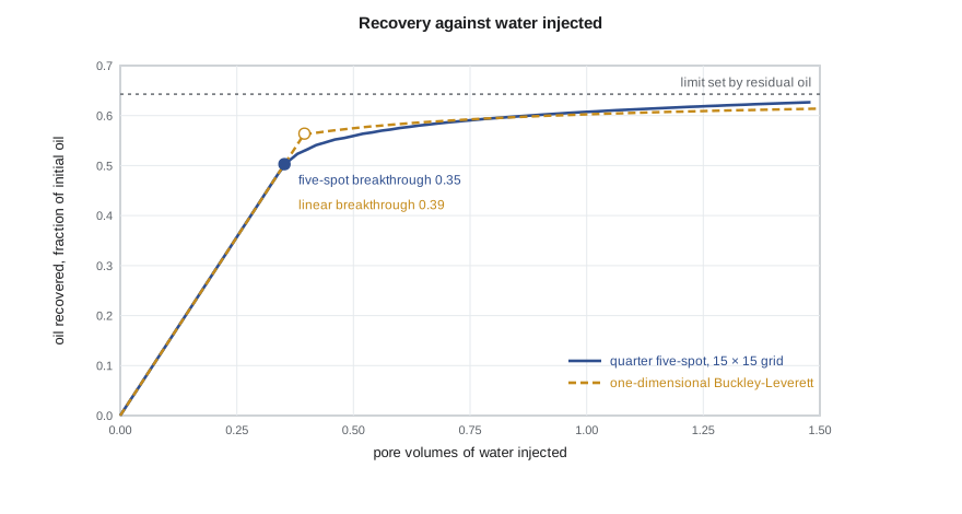
print(f"{c:3.1f} PV injected: {100 * rf:4.1f} percent of the starting oil produced")water breakthrough at 0.35 pore volumes injected 0.3 PV injected: 42.9 percent of the starting oil produced 0.6 PV injected: 57.5 percent of the starting oil produced 1.0 PV injected: 60.7 percent of the starting oil produced 1.5 PV injected: 62.7 percent of the starting oil produced
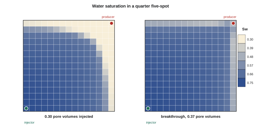
Water breaks through at about 0.35 pore volumes injected, earlier than the one-dimensional Buckley-Leverett value of about 0.40. Two effects combine. Flow in the five-spot converges toward the producer, so the front reaches the producer along the direct diagonal before the corners of the pattern are swept; the areal sweep at breakthrough is less than one. The coarse grid also adds numerical dispersion, as Lesson 9 showed, and five-point connections favor flow along the grid axes. Recovery continues after breakthrough as the swept area grows and water cut rises, reaching about 61 percent of the oil initially in the pattern after one pore volume. That is close to the maximum allowed by the residual oil saturation, because this idealized pattern is homogeneous and has a favorable mobility ratio. The real pilot, with its thief layer, recovers much less at the same injected volume.
Comparing the pattern with one dimension
Comparing the two-dimensional result with the one-dimensional solution separates displacement efficiency from sweep. Behind the front, both systems leave the same saturations, set by the fractional flow curve. What differs is how much of the pattern the front has contacted. In the one-dimensional system, the whole length is contacted at breakthrough. In the five-spot, only part of the area is, and the rest is contacted gradually afterward as streamlines through the corners carry water. Classic laboratory and analytical studies of the five-spot report areal sweep at breakthrough of around 70 percent for unit mobility ratio, rising slightly for favorable ratios and falling sharply for unfavorable ones.
Ethan's coarse model does not reproduce those values cleanly. Numerical dispersion smears the front over several blocks, so at breakthrough water has reached most of the pattern but at saturations well below the Buckley-Leverett values behind a sharp front, and the injector and producer occupy whole blocks rather than points. Refining to 30 by 30 blocks moves the result closer to the published values but quadruples the work per step and halves the stable time step. This is the trade-off of every simulation study in miniature, and the reason Lena insisted on a fine cross-section to quantify grid effects in the pilot model.
The study
The pilot-area model has about 150,000 active cells, with 164 ft blocks areally and twelve layers, including a separate layer for the thin high-permeability streak and layers for the two shale breaks. Properties were upscaled from the geological model with flow-based methods, and the thief layer was kept at its fine-scale permeability. The model was initialized by equilibration with J-function-scaled capillary pressure curves and reproduced the volumetric oil in place within one percent after the saturation-height inconsistency of Lesson 8 was resolved. A shut-in test showed no drift.
The history match proceeded from pressure to fluid movement. The pool pressure was matched by the aquifer strength and a small pore volume adjustment, both within the range supported by volumetrics and material balance. Breakthrough at the first producer was matched by a permeability enhancement along a mapped channel in the thief layer between the injector and that well, and the water cuts at all four pilot producers improved together. Injection profile logs, which showed about three quarters of the injected water entering the thief layer, were matched without further change. An ensemble smoother then produced 100 matched models that span the remaining uncertainty in pore volume, aquifer strength, thief layer continuity and relative permeability endpoints.
Forecasts
The four development cases of Lesson 11 were run on every ensemble member. The expansion with producer conversions in a line-drive pattern and four infill producers gave the highest incremental oil, with a P50 of about 1.23 MMSTB over twenty years and a P90 to P10 range of about 0.79 to 1.71 MMSTB. Limiting water injection to the current battery water handling capacity reduced the P50 by about 15 percent, because the injectors could not replace voidage once water cuts rose. The model also showed that injecting into the thief layer at high rates would cycle water rapidly to the nearest producers, so the expansion case includes profile control: injectors completed with selective injection or treated with a conformance gel in the thief layer if profiles show the same behavior as the pilot.
| Case | P50 incremental oil | Key observation |
|---|---|---|
| Continue pilot only | Small | Pilot area continues to respond; rest of pool depletes toward bubble point |
| Expansion with conversions | About 85 percent of the best case | Pressure maintained across the pool |
| Expansion with conversions and infills | 1.23 MMSTB | Best case; infills capture oil between patterns |
| Best case limited by water handling | About 15 percent below the best case | Battery water capacity becomes a constraint |
Recommendations
Lena and Ethan's recommendation has four parts. First, approve the waterflood expansion with conversions and infill producers, phased so that the first conversions are in the area nearest the pilot, where the model is best constrained. Second, expand battery water handling capacity before water cuts reach the level at which the model shows injection becoming restricted, about three years after the expansion starts. Third, monitor the flood with injection profile logs, tracers in the first new injectors and regular pressure surveys, and update the history match every year, so that the later phases can be adjusted if the thief layer proves more or less continuous than the P50 model assumes. Fourth, book the pilot-area waterflood volumes as reserves under the SEC rules and SPE-PRMS, and carry the expansion volumes as contingent resources until the project is approved and the first phase has responded.
At the presentation, the vice-president of development asks the question every simulation engineer expects: how sure are you? Ethan answers with the ensemble. The P90 case still justifies the first phase, the main uncertainty is the continuity of the thief layer, and the monitoring plan is designed to resolve it before the money for the later phases is committed. Lena adds that the model will be wrong in details, as all models are, but that it is the best tool available for deciding where to put the injectors, and that each year of flood data will make it better.
What the course has covered
The course began with the observation that a simulator is many small material balances joined by Darcy's law. It then built that machine piece by piece: the black-oil equations; finite-volume discretization and transmissibility; explicit, implicit and IMPES time stepping; Newton-Raphson iteration and preconditioned linear solvers; the Peaceman well model; grid design and upscaling; initialization by equilibration; and the numerical behavior of two-phase fronts. It then used the machine as engineers do, matching it to history, forecasting with ensembles and turning the results into decisions and reserves. Each of these steps appears in every commercial simulator, whatever its interface, and an engineer who understands them can read a run log, question a result and explain a forecast with confidence.
Worked problem
Voidage replacement for the expansion
After the expansion, the producers in one pattern are forecast to produce 252 STB/d of oil and 377 bbl/d of water, with B_o = 1.29 and B_w = 1.01. Free gas production is negligible because the pressure is above the bubble point. What water injection rate gives a voidage replacement ratio of 1.0?
Show solution
- The reservoir voidage is q_o B_o + q_w B_w = 252 × 1.29 + 377 × 1.01 = 325 + 381 = 706 rb/d.
- Injected water occupies B_w times its surface volume in the reservoir, so the injection rate for a ratio of 1.0 is 706 / 1.01 = 699 bbl/d.
- As water cut rises, the same reservoir voidage contains more water and less oil, so the injection requirement stays roughly constant while oil production falls.
Answer: About 699 bbl/d of injection is needed in this pattern for a voidage replacement ratio of 1.0. Summed over all patterns, this sets the water supply and handling capacity the expansion needs.
Common mistakes
MistakePresenting one matched model as the forecast.
InsteadPresent the ensemble range and explain which uncertainties drive it.
MistakeBooking expansion volumes as reserves before approval and response.
InsteadCarry them as contingent resources until the project is committed and supported by performance.
MistakeIgnoring facility constraints in the forecast.
InsteadInclude water handling and injection capacity as group controls; they can limit recovery.
MistakeTreating the study as finished at approval.
InsteadUpdate the model with surveillance data each year and adjust later phases.
Summary and key terms
- A quarter five-spot simulator combines finite volumes, IMPES, an iterative pressure solver and upstream-weighted saturation transport.
- Pattern floods break through earlier than one-dimensional floods because areal sweep at breakthrough is less than one.
- Coarse grids add numerical dispersion and orientation effects, so grid sensitivity must be checked.
- The pilot study built, initialized and matched a model, then forecast development cases with an ensemble.
- Recommendations combine the forecast range with facility constraints, monitoring plans and reserves rules.
- A simulation model is a living tool, updated as new data arrive.
- Five-spot pattern
- A waterflood pattern with an injector at the center of a square of producers, or the reverse.
- Areal sweep efficiency
- The fraction of the pattern area contacted by the injected fluid.
- Successive over-relaxation
- An iterative linear solver that accelerates Gauss-Seidel updates with a relaxation factor.
- Voidage replacement ratio
- Reservoir volume injected divided by reservoir volume produced.
- Line drive
- A waterflood pattern with rows of injectors alternating with rows of producers.
- Conformance control
- Treatments or completions that reduce flow into high-permeability layers to improve sweep.
- Surveillance
- Ongoing monitoring of a flood with logs, tracers, surveys and production data.
Practice problems
Work each problem on paper first, then reveal the answer to check.
Why can a quarter of a five-spot represent the whole pattern?
Show answer
By symmetry, the no-flow lines between wells divide the pattern into identical quarters.
Why is areal sweep at breakthrough less than one?
Show answer
Flow converges toward the producer, so the front reaches it along the diagonal before the corners are swept.
Why include water handling as a group control?
Show answer
If the battery cannot handle the produced water, injection and production must be restricted, reducing recovery.
How should expansion volumes be classified before approval?
Show answer
As contingent resources, moving to reserves once the project is committed and supported.
Lesson quiz · 5 questions
Score 60% or more to complete this lesson.
Create a free account to save your progress, take quizzes and earn a certificate.