
PET-420 · Lesson 8 of 12 · 19 min
Initialization and equilibration
Before the model can be matched against production, it must start from the right place: the pressures and saturations the pool had before the first well produced. This step, called initialization, decides the oil in place, the position of the contacts and the shape of the transition zone. Ethan's first initialization of the pilot model gives an oil in place six percent higher than the volumetric estimate, and when he runs the model for a year with every well shut in, the saturations in the lower layers creep downward and the pressures drift. Lena is not surprised. 'An initialization that moves with the wells shut in is not an equilibrium,' she says. 'Find out why before you do anything else.'
Hydrostatic equilibrium
In a reservoir that has been undisturbed for geological time, the fluids are at rest. There is no flow, so the potential of each phase is uniform within the connected region it occupies. That means each phase pressure varies with depth according to its own density:
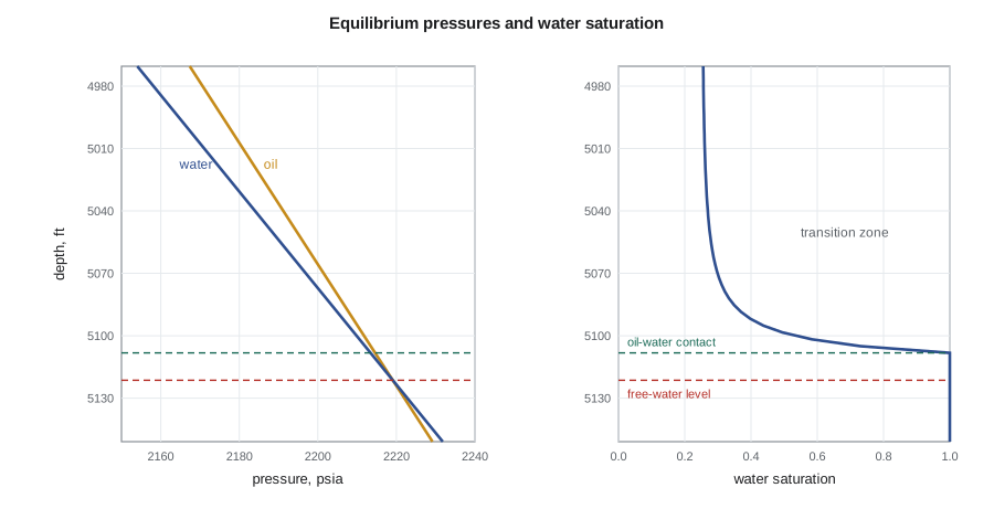
In the oil zone, the oil pressure increases with depth at the oil gradient; in the water zone, the water pressure increases at the water gradient. The two pressure lines meet at the free-water level, the depth at which the oil-water capillary pressure is zero. Above it, the oil pressure exceeds the water pressure by the capillary pressure, which grows linearly with height above the free-water level:
Equilibration in a simulator uses exactly this relation. The engineer gives a datum depth and pressure, the depth of the free-water level or of the oil-water contact and the depths of any gas-oil contact. The simulator integrates the phase pressure gradients up and down from the datum, using the fluid densities at each pressure, computes the capillary pressure at each depth and inverts the capillary pressure curve of each block's rock type to find its water saturation.
Free-water level and oil-water contact
The free-water level and the oil-water contact are not the same depth. The contact seen in wells, where the water saturation from logs rises to 100 percent, lies above the free-water level by the height corresponding to the capillary entry pressure, the minimum capillary pressure needed for oil to enter the largest pores. In high-permeability rock with a low entry pressure, the difference is small. In tight rock it can be several meters, and different rock types in the same pool show different apparent contacts above a single free-water level. Simulators that are given an oil-water contact usually treat it as the depth where capillary pressure is zero unless told otherwise, so the engineer must be clear which of the two is meant.
Above the contact lies the transition zone, in which water saturation falls from 100 percent toward the irreducible value as height increases. Its thickness depends on the capillary pressure curve and the density difference. A pool with light oil, a large density contrast and high-permeability rock has a thin transition zone; heavy oil in tight rock can have a transition zone tens of meters thick that holds a large fraction of the oil in place.
# Initialization: pressure and water saturation versus depth from the free-water level
SI = False
if SI:
    fwl, g_o, g_w, p_fwl, unit, pu, cu = 1561.0, 7.75, 9.75, 15300.0, "m", "kPa", "kPa"   # m, kPa/m, kPa/m, kPa
    depths = [1525, 1535, 1545, 1550, 1555, 1561]
else:
    fwl, g_o, g_w, p_fwl, unit, pu, cu = 5121.0, 0.343, 0.431, 2219.0, "ft", "psia", "psi"
    depths = [5003, 5036, 5069, 5085, 5102, 5121]
swirr, pd, lam = 0.25, 8.0, 2.0          # irreducible water, entry pressure (kPa), Brooks-Corey exponent
def pc_to_sw(pc_kpa):
    if pc_kpa <= pd: return 1.0
    return swirr + (1 - swirr) * (pd / pc_kpa) ** lam
for z in depths:
    hgt = fwl - z                                  # height above the free-water level
    pw = p_fwl - g_w * hgt                          # water pressure
    po = p_fwl - g_o * hgt                          # oil pressure
    pc = po - pw                                    # capillary pressure = (g_w - g_o) * height
    pc_kpa = pc if SI else pc / 0.145038
print(f"depth {z:5.0f} {unit}: oil {po:7.0f} {pu}, water {pw:7.0f} {pu}, Pc {pc:5.1f} {cu}, Sw {pc_to_sw(pc_kpa):.2f}")depth 5003 ft: oil 2179 psia, water 2168 psia, Pc 10.4 psi, Sw 0.26 depth 5036 ft: oil 2190 psia, water 2182 psia, Pc 7.5 psi, Sw 0.27 depth 5069 ft: oil 2201 psia, water 2197 psia, Pc 4.6 psi, Sw 0.30 depth 5085 ft: oil 2207 psia, water 2203 psia, Pc 3.2 psi, Sw 0.35 depth 5102 ft: oil 2212 psia, water 2211 psia, Pc 1.7 psi, Sw 0.61 depth 5121 ft: oil 2219 psia, water 2219 psia, Pc 0.0 psi, Sw 1.00
In the pool example, the oil and water gradients differ by about 0.088 psi/ft. With an entry pressure of 1.2 psi, the oil-water contact lies about 13 ft above the free-water level. Water saturation falls quickly through the next several meters and approaches irreducible within about 65 ft, so the lower simulation layers of the model lie partly in the transition zone. Their oil saturation, and therefore the oil in place, depends directly on the capillary pressure curve used.
Capillary pressure and rock type
Laboratory capillary pressure curves are measured on small core plugs, often with air and mercury or air and brine rather than reservoir fluids. Before use in a model they must be converted to reservoir conditions using the interfacial tension and contact angle of each fluid pair, and they must be related to the rock properties of each block. The Leverett J-function is the standard tool. It combines capillary pressure with the square root of permeability over porosity, so that curves from plugs of different quality collapse onto a single dimensionless curve for each rock type:
Each block then gets a capillary pressure curve scaled to its own permeability and porosity. High-permeability blocks receive low capillary pressures and low water saturations; tight blocks receive high capillary pressures and high water saturations. This reproduces the common observation that water saturation from logs correlates with rock quality at a given height above the free-water level.
A frequent source of trouble is inconsistency between the saturation-height model the petrophysicist used to compute water saturation from logs and the capillary pressure curves in the simulator. If the two disagree, the simulator's equilibrated saturations will not match the log-based saturations, and the oil in place will differ from the static model. Ethan's six percent discrepancy turns out to come from this. The static model used a saturation-height function fitted to logs, while the first version of the simulation used an unscaled laboratory curve from a single plug of better-than-average rock.
Non-equilibrium initialization
An alternative is to read the water saturation of each block directly from the static model rather than computing it from capillary pressure. This honors the petrophysical saturation exactly, but the resulting state is generally not in capillary equilibrium with the simulator's own curves. When the model is run, fluids move to restore equilibrium even with all wells shut in, and the pressures and saturations drift. Some simulators correct this by scaling the capillary pressure curve of each block so that the given saturation is in equilibrium at its height, a technique sometimes called Pc scaling or capillary pressure adjustment. It keeps the saturations and removes the drift, at the cost of block-by-block capillary curves that may look strange.
Whichever method is used, the standard test is the same: run the initialized model for a year or more with all wells shut in and confirm that pressures and saturations stay constant. Lena also checks that the initial oil, gas and water in place agree with the static model and with the material balance, region by region, and that the initial pressure at each well matches the first pressure measurement or drill-stem test.
| Check | What it confirms | Typical tolerance |
|---|---|---|
| Shut-in run of one year or more | Model is in equilibrium | No visible change in pressure or saturation |
| Oil in place against static model | Saturation-height and pore volume are consistent | Within one or two percent by region |
| Oil in place against material balance | Connected volume is right | Within the material balance uncertainty |
| Initial pressure at wells | Datum, gradients and contacts are right | Within gauge accuracy |
| Contacts against logs | Free-water level and entry pressure are consistent | Within a meter or so |
Several equilibrium regions
Real pools often have more than one free-water level. Faults that seal, or stratigraphic compartments separated by shales, can trap fluids at different contacts and pressures. Each such compartment is assigned its own equilibration region with its own datum pressure and contact depths. Neighboring regions with different pressures will try to equalize if they are connected in the model, so a transmissibility multiplier of zero across a sealing fault is often needed to keep them in equilibrium. Pools with a gas cap need a gas-oil contact as well, with the gas-oil capillary pressure setting the gas saturation in the gas-oil transition zone. In some deep pools the bubble point varies with depth, which is handled with a bubble point versus depth table.
Worked problem
Height of the oil-water contact above the free-water level
Oil and water densities at reservoir conditions are 49.3 and 62.1 lb/ft³. The capillary entry pressure at reservoir conditions is 1.16 psi. How high above the free-water level is the oil-water contact? What is the capillary pressure 65.6 ft above the free-water level?
Show solution
- The pressure gradient difference is (62.1 − 49.3) / 144 = 0.089 psi/ft.
- The contact lies where P_c equals the entry pressure: h = 1.16 / 0.089 = 13 ft above the free-water level.
- At 65.6 ft above the free-water level, P_c = 0.089 × 65.6 = 5.8 psi.
Answer: The oil-water contact is about 13 ft above the free-water level, and the capillary pressure at 65.6 ft above it is about 5.8 psi.
Initialization of the pilot model
Once the capillary pressure problem is found, Ethan replaces the single laboratory curve with J-function curves for each of the three rock types, fitted to the same capillary pressure data the petrophysicist used for the saturation-height model. The equilibrated oil in place falls to within one percent of the static model in every region, and the simulated water saturation profiles at each well agree with the log-derived profiles through the transition zone. A two-year run with all wells shut in shows no change in pressure or saturation at any block, so the model is in equilibrium.
Ethan then compares the initial pressures with the pool's earliest measurements. The discovery well's drill-stem test recorded a pressure of 2,219 psia at the free-water level datum, and the initialized model reproduces it exactly because that is how the datum was set. The real test is the second and third wells, drilled before significant production, whose first pressure surveys were taken at different depths. The model matches both within 3 psi, confirming that the oil gradient and the contact depth are consistent. Lena has seen models in which a datum pressure was entered at the wrong depth, and every subsequent pressure was offset by the hydrostatic head of the difference. That kind of error is invisible in the shut-in test and only shows up when initial pressures are checked against the measurements.
Two smaller decisions complete the initialization. The analytical aquifer is attached to the bottom layer of the blocks along the lower edge of the model, with its initial pressure equal to the water pressure at that depth so that it starts in equilibrium with the reservoir. The water above the contact in the transition zone is mobile in the model only where its saturation exceeds the critical water saturation of the relative permeability curves; below that it is immobile even though it is above irreducible. Ethan checks that the endpoint scaling gives consistent critical saturations in every rock type, because an inconsistency there would let the transition zone produce water as soon as the wells opened, a behavior the early production history does not show.
Common mistakes
MistakeTreating the oil-water contact and the free-water level as the same depth.
InsteadThe contact lies above the free-water level by the entry pressure height.
MistakeUsing an unscaled laboratory capillary pressure curve for every block.
InsteadScale curves to each block's permeability and porosity with the J-function.
MistakeSkipping the shut-in equilibrium test.
InsteadRun the model with wells shut in and confirm nothing moves before matching history.
MistakeConnecting compartments with different contacts.
InsteadUse separate equilibration regions and seal the faults between them if they are not in communication.
Summary and key terms
- Initialization places the fluids in gravity-capillary equilibrium, with uniform phase potentials.
- Phase pressures follow their density gradients and meet at the free-water level, where capillary pressure is zero.
- Capillary pressure grows with height above the free-water level and converts to water saturation through each rock type's curve.
- The oil-water contact lies above the free-water level by the entry pressure height.
- The J-function scales capillary pressure to each block's permeability and porosity.
- A shut-in run, oil in place comparisons and initial pressure checks confirm the initialization before history matching.
- Initialization
- Setting the starting pressures and saturations of every block in a simulation model.
- Equilibration
- Initialization by gravity-capillary equilibrium from datum pressures and contact depths.
- Free-water level
- The depth at which oil-water capillary pressure is zero.
- Oil-water contact
- The depth below which the rock is fully water saturated, above the free-water level by the entry height.
- Transition zone
- The interval above the contact in which water saturation falls from one to irreducible.
- Leverett J-function
- A dimensionless capillary pressure that combines Pc with the square root of k over φ.
- Equilibration region
- A part of the model with its own datum pressure and contacts.
Practice problems
Work each problem on paper first, then reveal the answer to check.
Why are phase potentials uniform at initial conditions?
Show answer
The fluids are at rest, so there is no potential gradient to drive flow.
What sets the thickness of a transition zone?
Show answer
The capillary pressure curve and the density difference between the phases.
Why might a non-equilibrium initialization drift with all wells shut in?
Show answer
The given saturations are not in equilibrium with the simulator's capillary pressure curves.
How do you represent two compartments with different contacts?
Show answer
Separate equilibration regions, usually separated by a sealing fault with zero transmissibility multiplier.
Lesson quiz · 5 questions
Score 60% or more to complete this lesson.
Create a free account to save your progress, take quizzes and earn a certificate.