
PET-420 · Lesson 11 of 12 · 20 min
Forecasting, uncertainty and reserves
A matched model is a tool, not a result. Management's question is still the one Lena was asked at the start: should Prairie Crest expand the waterflood to the whole Mission Canyon pool, and how much oil would that add? Answering it means running the model forward under different development plans, measuring the uncertainty in each forecast and translating the results into the language of reserves and economics. 'The forecast is where the model earns its keep,' Lena says, 'and it is also where people trust it too much. Our job is to give them a range they can make decisions with.'
Prediction cases
A forecast starts from the end of the history match, with the reservoir state the match has produced. From there, the model is run under a set of cases, each a plausible way of developing and operating the pool. The base case, sometimes called the do-nothing or no-further-activity case, continues current operations with no new investment. Development cases add the investments being considered. Ethan and Lena define four: continuing the pilot alone; expanding the flood with conversions of existing producers to injectors in a line-drive pattern; expanding with conversions and four new infill producers; and the same expansion with injection limited by water handling capacity at the battery.
In a forecast, wells are controlled differently from history. Producers usually run at a bottomhole pressure set by their artificial lift, with limits on maximum liquid rate and economic limits on minimum oil rate or maximum water cut, beyond which they are shut in or worked over. Injectors run at a target rate, often set to replace the reservoir voidage of the producers in their pattern, with a maximum bottomhole pressure below fracture pressure. Group controls represent shared constraints: the total water the battery can handle, the total injection the water plant can supply and the gas the compressor can take.
The incremental value of a project is the difference between a development case and the base case, not the total production of the development case. For the expansion, the increment includes both oil the flood recovers that primary depletion could not, and oil recovered sooner because the pressure is maintained. Both matter to the economics. Simulation shows both in the same run, which is one of its main advantages over simpler methods.
Sources of uncertainty
Every forecast inherits uncertainty from three sources. The first is the reservoir description: oil in place, the continuity and permeability of the thief layer, the aquifer, the relative permeability curves and many other quantities that the history match has narrowed but not fixed. The second is the model itself: grid resolution, numerical dispersion, the black-oil fluid description and the well model all introduce errors, some quantifiable and some not. The third is the future: well performance, facility uptime, operating decisions and prices that no reservoir model can predict.
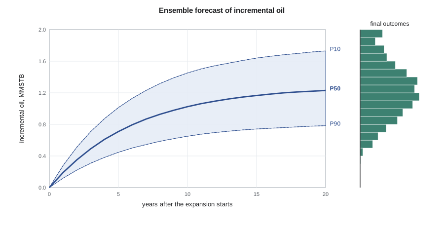
The usual way to express reservoir uncertainty is an ensemble of forecasts. Each member uses a different combination of the uncertain parameters, chosen so that all members are consistent with the history. The spread of the ensemble's results is a measure of the forecast uncertainty. Three statistics summarize it: P90, the value exceeded by 90 percent of members, a low estimate; P50, the median; and P10, the value exceeded by only 10 percent, a high estimate. Under the probabilistic definitions used in reserves evaluation, these correspond broadly to the proved, proved plus probable and proved plus probable plus possible categories.
The code below builds such an ensemble for the full-field expansion in its simplest form. Oil in place comes from the distribution left by the history match. Displacement efficiency behind the front and volumetric sweep, which together give the recovery factor of the flood, are drawn from ranges based on the core data and the pilot's performance. The primary and aquifer recovery factor is held at a fixed value, and the increment is the oil in place times the difference between the flood and the base recovery factors.
# Ensemble forecast of waterflood incremental oil: P90, P50 and P10
import random, math
SI = False
random.seed(11)
n = 2000
N50 = 5.11e6 if SI else 8.49e6 / 6.28981                   # median oil in place, m3
results = []
for _ in range(n):
    N = random.lognormvariate(math.log(N50), 0.10)           # oil in place (history-matched ensemble)
    ed = random.uniform(0.52, 0.62)                          # displacement efficiency behind the front
    ev = random.triangular(0.45, 0.75, 0.62)                 # volumetric sweep (areal x vertical)
    base = 0.20                                              # primary plus aquifer recovery factor
    rf = max(ed * ev, base)                                  # recovery factor with the flood
    results.append(N * (rf - base))
results.sort()
p90, p50, p10 = (results[int(n * q)] for q in (0.10, 0.50, 0.90))   # P90 is exceeded by 90 percent of cases
f, u = (1e-6, "million m3") if SI else (6.28981e-6, "MMSTB")
print(f"incremental oil: P90 {p90 * f:.2f}, P50 {p50 * f:.2f}, P10 {p10 * f:.2f} {u}")
print(f"mean {sum(results) / n * f:.2f} {u}; P10/P90 ratio {p10 / p90:.2f}")
print(f"chance the flood adds less than {0.5 if SI else 0.8} {u}: "
f"{100 * sum(1 for r in results if r * f < (0.5 if SI else 0.8)) / n:.0f} percent")incremental oil: P90 0.79, P50 1.23, P10 1.71 MMSTB mean 1.25 MMSTB; P10/P90 ratio 2.17 chance the flood adds less than 0.8 MMSTB: 10 percent
The ensemble gives a P50 increment of about 1.23 MMSTB with a P90 to P10 range of about a factor of two. The ratio of P10 to P90 is a common summary of how uncertain a forecast is; values around two to three are typical for a waterflood with a pilot, while frontier projects can show ratios of ten or more. The ensemble also answers the question managers often care about most: the chance that the flood adds less than a threshold volume, here about 10 percent. In the full study, each member is a complete simulation run rather than a formula, but the logic is the same.
Sampling and experimental design
Running a full simulation for every one of thousands of combinations is rarely possible. Engineers therefore use designs that sample the parameter space efficiently. A tornado chart, made by moving each parameter alone from its low to its high value with the others at their base values, shows which parameters matter most and is a standard first step. Experimental designs, such as Plackett-Burman screening and Box-Behnken or Latin hypercube sampling, choose a few tens of runs that cover the space and allow interactions between parameters to be estimated. Response surfaces fitted to those runs act as fast proxies for Monte Carlo sampling. With modern computing, many studies now run ensembles of a hundred or more full models directly, often the same ensemble produced by an ensemble history match.
Two cautions apply. First, the ensemble is only as wide as the uncertainty put into it; a parameter left fixed contributes nothing to the spread, however uncertain it really is. Second, some uncertainties are scenarios rather than continuous ranges: the thief layer either extends across the pool or does not, and a fault either seals or leaks. Such alternatives are best handled as separate scenarios, each with its own matched ensemble, so that one does not average away a possibility that would change the development plan.
From forecasts to reserves
Simulation forecasts feed reserves evaluations, which in North Dakota follow the SEC rules and SPE-PRMS. Reserves are the remaining quantities expected to be recovered commercially from known accumulations under defined conditions. They are classified by certainty into proved, probable and possible. For a waterflood expansion, the regulations and guidelines generally require that improved recovery reserves be supported by a successful pilot or by analogous projects in similar reservoirs, that the project be approved or committed and that the engineering basis be documented. The Mission Canyon waterflood pilot provides exactly this support, which is why the original plan recommended booking waterflood volumes only after the pilot had performed.
Reserves can be estimated deterministically, by choosing low, best and high cases, or probabilistically, from distributions such as the ensemble above, in which case proved reserves correspond to at least a 90 percent probability that the recovered quantity will equal or exceed the estimate. Either way, the evaluator must reconcile simulation results with the other evidence: decline analysis of the existing wells, material balance and analog recovery factors. A simulation forecast that is far outside the range of analogs needs a clear explanation, not just a matched model.
| Category | Probabilistic meaning | Typical evidence for a waterflood increment |
|---|---|---|
| Proved (1P) | At least 90 percent chance of meeting or exceeding | Successful pilot response in the same pool, committed project |
| Proved plus probable (2P) | At least 50 percent chance | Pilot response extrapolated to the expansion area |
| Proved plus probable plus possible (3P) | At least 10 percent chance | Favorable sweep and oil in place assumptions |
| Contingent resources | Not yet commercial or not committed | Flood expansion before approval or funding |
Forecasting unconventional wells
The same principles apply to the multistage fractured horizontal wells that dominate tight oil development, but the emphasis shifts. Their production is controlled by the fracture geometry and the stimulated rock around each stage rather than by interwell displacement, and their long transient flow periods make simple decline curves unreliable early in life. Simulation of a few representative wells, matched to their early production and pressure data, is used to calibrate type curves for the rest. In the Bakken and similar plays, operators have also simulated enhanced recovery by gas injection, in which one well cycles between injection and production, to judge whether pilots are worth the investment. The ensemble and scenario ideas carry over directly, with completion design and fracture properties added to the uncertain parameters.
Worked problem
Reading an ensemble
An ensemble of 2,000 forecasts of incremental oil is sorted from lowest to highest. The 200th value is 0.79 MMSTB, the 1,000th is 1.23 MMSTB and the 1,800th is 1.71 MMSTB. Identify P90, P50 and P10 and compute the P10/P90 ratio.
Show solution
- P90 is exceeded by 90 percent of members, so it is the value with 10 percent of members below it: the 200th, 0.79 MMSTB.
- P50 is the median, the 1,000th value: 1.23 MMSTB.
- P10 is exceeded by only 10 percent: the 1,800th value, 1.71 MMSTB. The ratio P10/P90 = 1.71 / 0.79 ≈ 2.2.
Answer: P90, P50 and P10 are about 0.79, 1.23 and 1.71 MMSTB, and the P10/P90 ratio is about 2.2, a moderate uncertainty typical of a piloted waterflood.
Economics and decisions
Reservoir engineers rarely make the final decision; they supply the forecasts on which it rests. The ensemble's oil profiles become cash flow forecasts once the economics group applies prices, operating costs, capital costs, royalties and taxes. The usual measures are net present value at a corporate discount rate, rate of return and payback time. Because each ensemble member produces its own profile, the economics can also be calculated member by member, giving a distribution of net present value rather than a single number. That distribution often shows something the oil forecast alone does not: a case with a higher P50 oil increment may have a lower expected value if it needs more capital up front or delays production.
Ensembles also support decisions about information. The value of information is the improvement in the expected outcome that a measurement would bring by changing the decision in some outcomes. In the pilot study, Ethan and Lena ask whether a tracer program in the first expansion injectors, at a modest cost, is worth running. The ensemble shows that the tracer arrival times would distinguish the models with a continuous thief layer from those with a discontinuous one, and that the second phase of the expansion would be designed differently in the two cases. The tracers therefore have real value, and they are included in the monitoring plan.
Finally, every forecast should be documented so that it can be reproduced and compared with what actually happens. Lena keeps the forecast ensembles from every earlier study of the pool. Comparing a five-year-old forecast with the actual production since then is the best calibration of how far the group's forecasts can be trusted, and it is a check that many organizations skip.
Common mistakes
MistakeReporting the total production of a development case as its value.
InsteadReport the increment over a base case run from the same matched state.
MistakeConfusing P90 with the high estimate.
InsteadP90 is the low estimate, exceeded by 90 percent of outcomes.
MistakeLeaving uncertain parameters fixed in the ensemble.
InsteadEvery important uncertainty must be sampled, or the spread will be too narrow.
MistakeAveraging distinct geological scenarios together.
InsteadTreat alternatives such as a sealing or leaking fault as separate scenarios.
Summary and key terms
- Forecasts run the matched model forward under base and development cases with realistic well and facility controls.
- The value of a project is its increment over a base case, including both added and accelerated oil.
- Forecast uncertainty comes from the reservoir description, the model itself and future operations.
- Ensembles of matched models give P90, P50 and P10 forecasts; the P10/P90 ratio summarizes the spread.
- Tornado charts, experimental designs and proxies make uncertainty analysis affordable.
- Simulation forecasts support reserves under the SEC rules and SPE-PRMS, which require evidence such as a successful pilot for waterflood reserves.
- Base case
- A forecast with current operations continued and no new investment.
- Incremental recovery
- The additional oil from a project, measured against the base case.
- P90
- A low estimate that 90 percent of outcomes are expected to equal or exceed.
- P10
- A high estimate that only 10 percent of outcomes are expected to equal or exceed.
- Tornado chart
- A chart showing the effect of each parameter moved alone between its low and high values.
- Experimental design
- A planned set of simulation runs chosen to cover the parameter space efficiently.
- Contingent resources
- Discovered quantities not yet commercial or committed, such as an unapproved flood expansion.
Practice problems
Work each problem on paper first, then reveal the answer to check.
Why is a base case needed?
Show answer
The project's value is its increment over continuing current operations from the same starting state.
What does a P10/P90 ratio of 2.2 tell you?
Show answer
The high estimate is about 2.2 times the low one, a moderate uncertainty.
Why should a sealing and a leaking fault be separate scenarios?
Show answer
They are distinct alternatives that may change the plan; averaging hides that.
What evidence usually supports waterflood reserves?
Show answer
A successful pilot in the same pool or analogous projects, with a committed project.
Lesson quiz · 5 questions
Score 60% or more to complete this lesson.
Create a free account to save your progress, take quizzes and earn a certificate.