
PET-420 · Lesson 3 of 12 · 19 min
Finite differences and transmissibility
The equations of Lesson 2 are partial differential equations: they hold at every point of the reservoir and every instant of time. A computer cannot solve them at infinitely many points, so the simulator replaces them with algebraic equations that hold for a finite number of blocks and a finite number of time steps. This step is called discretization. Almost every commercial simulator uses the finite-volume method on a grid of blocks, often described with the older name of finite differences. Lena gives Ethan a small exercise before he sees the full model: build a one-dimensional row of ten blocks between the injector and a producer, write the flow between each pair of blocks by hand and solve it. 'Once you have done ten blocks on paper,' she says, 'a million blocks are only bookkeeping.'
From derivatives to differences
A derivative is the limit of a ratio of differences. The first step of discretization is to stop before the limit and use the difference itself. If pressure is known at the centers of two adjacent blocks, i and i + 1, separated by a distance Δx, the pressure gradient at the face between them is approximately:
This central difference is accurate to second order in Δx: halving the block size reduces the error by about a factor of four, as long as the pressure varies smoothly. The second derivative, which appears in the diffusivity equation, becomes the difference of two such face gradients divided by Δx, giving the familiar three-point formula p_{i−1} − 2p_i + p_{i+1} over Δx squared. Taylor series expansions show where the error comes from and how it scales, and they are the standard tool for analyzing the accuracy of any difference scheme.
The finite-volume view
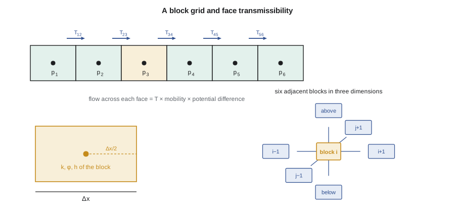
Engineers usually prefer a more physical derivation. Treat each block as a small tank with a definite pore volume. Integrate the mass balance over the block: the accumulation term becomes the change in fluid mass in the block, the divergence term becomes the sum of the flows across its faces and the source term becomes the well rate. Then approximate each face flow with Darcy's law using the pressures in the two blocks that share the face. The result for block i in one dimension, for a single incompressible phase, is:
This form makes conservation exact. Whatever leaves block i through a face enters its neighbor through the same face, so no fluid is created or lost between blocks, regardless of how coarse the grid is. The only approximation is in how the face flow depends on the two block pressures. That is a key reason the finite-volume method dominates reservoir simulation: oil in place and cumulative production always balance, a property engineers check routinely.
Transmissibility
The coefficient T in the equation above is the transmissibility of the face. It gathers the rock and geometry into one number per connection, multiplied by the phase mobility to give the flow rate per unit pressure difference. For a face between two blocks with the same permeability k, cross-sectional area A and center-to-center distance Δx, and a fluid of viscosity μ:
When the two blocks have different permeabilities, the face transmissibility must reflect the fact that fluid flows first through half of block i and then through half of block i + 1. The two halves act like resistances in series, so their resistances add. That gives the harmonic average:
The harmonic average is dominated by the smaller permeability. If one block is a shale with almost no permeability, the face between it and a sandstone block carries almost no flow, which is physically correct. An arithmetic average would wrongly let fluid pass through the barrier. Simulators usually compute geometric transmissibilities without the viscosity, store them for every connection and multiply by the phase mobility at each step, often with user-supplied multipliers to represent faults or baffles.
In field units a unit conversion constant appears, because Darcy's law in millidarcies, feet and pounds per square inch does not give barrels per day directly. In metric units with permeability in millidarcies, area in square meters, viscosity in millipascal seconds, length in meters and pressure in kilopascals, the constant is about 8.53 × 10⁻⁵ to give cubic meters per day. In field units it is 0.001127 to give reservoir barrels per day per pound per square inch, with permeability in millidarcies, area in square feet, viscosity in centipoise and length in feet.
A row of ten blocks
Ethan's exercise is a row of ten blocks, each 164 ft long, with a cross-section 1,312 ft wide and 21 ft thick, between a face held at the injector pressure and a face held at the producer pressure. The permeability varies along the row, including two blocks of a higher-permeability streak. Writing the block equation for each block gives ten linear equations. Each equation involves only the block itself and its two neighbors, so the matrix of coefficients is tridiagonal: non-zero only on the main diagonal and the two diagonals next to it.
A tridiagonal system can be solved directly in a number of operations proportional to the number of blocks with the Thomas algorithm, a streamlined form of Gaussian elimination. A forward sweep eliminates the lower diagonal, and back substitution recovers the pressures from the last block to the first. The code below sets up and solves the system, then checks the computed rate against the total resistance of the blocks in series.
# 1D incompressible flow between an injector block and a producer block, solved with the Thomas algorithm
SI = False
n, dx, area = 10, 50.0, 400 * 6.5           # blocks, block length (m), cross-section (m2)
k = [15, 15, 18, 40, 40, 12, 10, 15, 20, 15]  # permeability by block, mD
mu = 0.72                                    # mPa.s
c = 9.869e-16 * 1e3 / 1e-3 * 86400           # Darcy units: m3/d per (mD m2 kPa / (mPa.s m))
pL, pR = 15000.0, 12000.0                    # kPa held at the outer faces of block 1 and block n
def harm(a, b): return 2 * a * b / (a + b)
T = [c * harm(k[i], k[i + 1]) * area / (mu * dx) for i in range(n - 1)]
TL = c * k[0] * area / (mu * dx / 2); TR = c * k[-1] * area / (mu * dx / 2)
a = [0.0] * n; b = [0.0] * n; cc = [0.0] * n; d = [0.0] * n
for i in range(n):
    if i > 0: a[i] = -T[i - 1]; b[i] += T[i - 1]
    if i < n - 1: cc[i] = -T[i]; b[i] += T[i]
b[0] += TL; d[0] += TL * pL; b[-1] += TR; d[-1] += TR * pR
for i in range(1, n):                         # Thomas algorithm: forward sweep
    w = a[i] / b[i - 1]; b[i] -= w * cc[i - 1]; d[i] -= w * d[i - 1]
p = [0.0] * n; p[-1] = d[-1] / b[-1]
for i in range(n - 2, -1, -1): p[i] = (d[i] - cc[i] * p[i + 1]) / b[i]   # back substitution
q = T[0] * (p[0] - p[1])
R = mu * dx / 2 / (c * k[0] * area) + sum(1 / t for t in T) + mu * dx / 2 / (c * k[-1] * area)
f, pu, qf, qu = (1, "kPa", 1, "m3/d") if SI else (0.145038, "psia", 6.28981, "bbl/d")
print("block pressures:", " ".join(f"{x * f:.0f}" for x in p), pu)
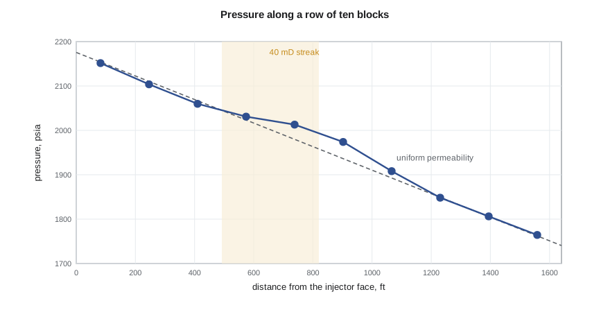
print(f"rate through the line: {q * qf:.2f} {qu}; series-resistance check: {(pL - pR) / R * qf:.2f} {qu}")block pressures: 2152 2104 2060 2031 2013 1974 1908 1848 1806 1764 psia rate through the line: 191.89 bbl/d; series-resistance check: 191.89 bbl/d
The rates agree to the last digit, which confirms that the scheme conserves mass and that the harmonic face averages are equivalent to adding resistances. The pressure profile is not a straight line: it falls slowly across the high-permeability blocks and steeply across the tighter ones, exactly as the flow through each must be the same. A geologist looking at the profile would see the streak immediately.
Two and three dimensions
In two and three dimensions each block has more neighbors. On a Cartesian grid, a block has four neighbors in two dimensions and six in three, and the matrix has five or seven non-zero diagonals. In the vertical direction the transmissibility uses the vertical permeability and the horizontal area of the block, and the potential difference includes gravity: the flow between two vertically stacked blocks depends on p_{i+1} − p_i − ρ g (D_{i+1} − D_i). Ignoring this term would make fluids flow upward or downward in a reservoir at rest.
Real reservoirs are not rectangular boxes. Corner-point grids let each block have arbitrary corner depths, so the grid can follow dipping layers, pinch-outs and faults. Across a fault, a block may connect to several blocks on the other side, with transmissibilities computed from the overlapping areas; these non-neighbor connections are why the matrix of a faulted model has entries far from the main diagonals. Unstructured grids made of triangular prisms or Voronoi polygons, sometimes called perpendicular bisector grids, follow wells and faults even more closely. On any of these grids, the finite-volume idea is unchanged: one mass balance per block, one transmissibility per connection.
| Grid type | Strength | Limitation |
|---|---|---|
| Cartesian, values at block centers | Simple, fast, easy to check | Cannot follow dipping or faulted geometry closely |
| Corner-point | Follows layers, pinch-outs and faults | Distorted cells reduce accuracy of the two-point flux |
| Radial | Natural near a single well | Only for single-well studies |
| Unstructured (Voronoi, prisms) | Fits wells, faults and fractures | Larger setup effort and less common workflows |
| Local grid refinement | Fine cells only where needed | Interfaces between fine and coarse cells need care |
One caution goes with all non-orthogonal grids. The two-point flux approximation used by most simulators, which writes each face flow from the two block pressures only, is exact only when the line joining the block centers is perpendicular to the face and the permeability tensor is aligned with the grid. On strongly distorted corner-point cells, or with strongly anisotropic permeability at an angle to the grid, it introduces a grid orientation error. Multipoint flux approximations reduce the error at the cost of a more complicated matrix, and are offered by several research and commercial codes.
Worked problem
A face transmissibility across a permeability contrast
Two adjacent blocks are each 164 ft long, with a face area of 27,990 ft². Block A has permeability 40 mD and block B has 12 mD. Oil viscosity is 0.72 cp. Find the face transmissibility and the oil rate for a pressure difference of 14.5 psi between block centers.
Show solution
- The series resistance is Δx/(2k_A) + Δx/(2k_B) = 25/40 + 25/12 in metric length units, giving 0.625 + 2.083 = 2.708; the effective permeability over the 50 m is 50 / 2.708 = 18.5 mD, the harmonic average of 40 and 12, well below the arithmetic average of 26 mD.
- In field units, T = 0.001127 × 18.46 × 27,990 / (0.72 × 164) = 4.93 rb/d per psi.
- The rate is T times the pressure difference: 4.93 × 14.5 = 71 rb/d.
Answer: The face transmissibility is about 4.9 rb/d per psi and the rate about 71 rb/d. The tighter block controls the flow.
Common mistakes
MistakeAveraging permeability arithmetically across a face.
InsteadUse the harmonic average for flow in series; the tighter block controls the face.
MistakeLeaving out the gravity term in vertical connections.
InsteadUse the potential difference, including ρ g ΔD, so a reservoir at rest stays at rest.
MistakeAssuming the two-point flux is exact on any grid.
InsteadIt is exact only on orthogonal grids aligned with the permeability; distorted cells add orientation error.
MistakeChecking a model only by eye.
InsteadCheck mass balance and compare a simple case with an analytical solution, as the series-resistance check does.
Summary and key terms
- Discretization replaces the differential equations with algebraic equations for a finite number of blocks and time steps.
- The finite-volume method writes an exact mass balance for each block and approximates only the face flows.
- Face flow equals transmissibility times mobility times the potential difference between the two blocks.
- Transmissibility across a permeability contrast uses the harmonic average, so barriers are honored.
- A one-dimensional system is tridiagonal and solved directly with the Thomas algorithm; three-dimensional systems have seven or more diagonals.
- Corner-point and unstructured grids follow geology more closely but strain the two-point flux approximation.
- Discretization
- Replacing continuous equations with algebraic equations on a grid of blocks and time steps.
- Finite-volume method
- A discretization that writes an integral mass balance for each block, conserving mass exactly.
- Transmissibility
- The rock and geometry factor that multiplies mobility and potential difference to give face flow.
- Harmonic average
- An average dominated by the smallest value, appropriate for resistances in series.
- Tridiagonal matrix
- A matrix with non-zero entries only on the main diagonal and the two adjacent diagonals.
- Corner-point grid
- A grid in which each cell is defined by its eight corner points, allowing dipping and faulted geometry.
- Non-neighbor connection
- A flow connection between blocks that are not adjacent in the grid indexing, for example across a fault.
Practice problems
Work each problem on paper first, then reveal the answer to check.
Why does the finite-volume method conserve mass exactly?
Show answer
Each face flow leaves one block and enters its neighbor, so nothing is lost between blocks.
Why is the harmonic average used for face transmissibility?
Show answer
The two half-blocks are resistances in series, and series resistances add.
How many non-zero diagonals does the matrix of a 3D Cartesian model have?
Show answer
Seven: the block itself and its six neighbors.
What does a transmissibility multiplier on a fault represent?
Show answer
A reduction in flow across the fault due to fault rock or juxtaposition, as estimated by the geologist.
Lesson quiz · 5 questions
Score 60% or more to complete this lesson.
Create a free account to save your progress, take quizzes and earn a certificate.