
PET-420 · Lesson 6 of 12 · 20 min
Well models and the Peaceman well index
A well is tiny compared with a grid block. The wellbore of a Mission Canyon pool producer is about 7 in across, while the blocks in Lena's pilot model are 164 ft on a side. The simulator cannot resolve the steep pressure drop that concentrates in the few meters around the well, yet that drop controls how much the well produces. The well model bridges the gap. It relates the flowing bottomhole pressure, which engineers measure and control, to the block pressure, which the simulator computes, and it is the part of the model that the history match most often has to adjust. Ethan's job this week is to connect the twenty pilot-area wells to the grid and understand every number in the connection.
Block pressure is not well pressure
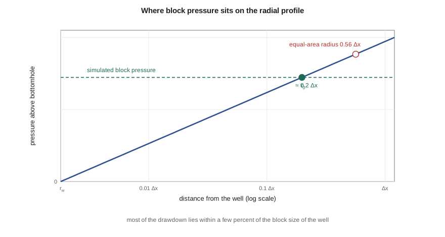
In a radial flow system around a well, pressure rises with the logarithm of distance. Most of the drawdown occurs close to the well: in a typical case, half of it is spent within a few meters. A grid block containing the well has a single pressure, which represents some kind of average over the block. That block pressure is far higher than the flowing bottomhole pressure and somewhat lower than the pressure at the edge of the drainage area. A well model must state precisely which radius the block pressure corresponds to.
The answer was given by Donald Peaceman, in a paper published in 1978 and extended in 1983. He solved the finite-difference equations for a single well in the center of a fine grid of square blocks and compared the numerical block pressure with the analytical radial solution. For steady radial flow toward a well in a square block of side Δx with uniform isotropic permeability, the computed block pressure equals the true flowing pressure at a radius:
This equivalent radius is much smaller than the radius of a circle with the same area as the block, about 0.56 Δx, which had been used by earlier modelers and overestimated well rates. Peaceman's result shows that block pressure in a numerical model is not the average pressure in the block, a point that matters every time simulated and measured pressures are compared.
The well index
With the equivalent radius known, the steady radial flow equation between r_0 and the wellbore radius r_w gives the relation between block pressure and bottomhole pressure:
The well index WI, also called the connection transmissibility factor, depends on permeability, completed thickness, the equivalent radius, the wellbore radius and the skin factor s. A unit conversion constant appears in practical units, the same one as in the transmissibility. In a layered model, each completed layer has its own connection with its own well index, and the well rate is the sum over connections. Bottomhole pressure is usually referred to a datum depth, and the pressure at each connection includes the hydrostatic head of the fluid in the wellbore between the datum and that connection.
For anisotropic permeability, with kx different from ky, Peaceman's formula uses the geometric mean permeability in the well index and an equivalent radius that depends on both block dimensions and both permeabilities:
Horizontal wells use the same formula with the directions rotated, so that the permeabilities and dimensions perpendicular to the well, usually horizontal and vertical, replace kx, ky, Δx and Δy. That is one reason horizontal well indices are more uncertain: vertical permeability is poorly known and the blocks are usually much thinner than they are wide.
How grid size affects the well
The code below computes the well index for a Mission Canyon pool producer in square blocks of four different sizes, holding block pressure and bottomhole pressure fixed. It then compares the result with the pseudosteady radial inflow formula from well performance work, which uses the average drainage-area pressure.
# Peaceman well index: connecting a well to a grid block
import math
SI = False
k, h, mu, Bo, rw, skin = 15.0, 6.5, 0.72, 1.29, 0.089, 2.0      # mD, m, mPa.s, rm3/sm3, m, dimensionless
c = 9.869e-16 * 1e3 / 1e-3 * 86400                         # m3/d per (mD m kPa / mPa.s)
p_block, p_wf = 13600.0, 9500.0                            # kPa
for dx in (25.0, 50.0, 100.0, 200.0):
    r0 = 0.198 * dx                                        # square block, isotropic permeability
    WI = 2 * math.pi * c * k * h / (math.log(r0 / rw) + skin)
    q = WI / (mu * Bo) * (p_block - p_wf)
    if SI:
        print(f"block {dx:5.0f} m: r0 = {r0:5.1f} m, WI = {WI:6.4f}, oil rate {q:5.1f} m3/d")
    else:
        print(f"block {dx * 3.28084:5.0f} ft: r0 = {r0 * 3.28084:5.1f} ft, WI = {WI * 6.28981 / 0.145038:6.3f} (field), oil rate {q * 6.28981:6.1f} STB/d")
# block pressure is not the drainage-boundary pressure: compare with the radial formula from PET-320
re_ = 400.0
q_rad = 2 * math.pi * c * k * h * (p_block - p_wf) / (mu * Bo * (math.log(re_ / rw) - 0.75 + skin))
print(f"pseudosteady radial formula with average pressure = block pressure: {q_rad:.1f} m3/d" if SI else
f"pseudosteady radial formula with average pressure = block pressure: {q_rad * 6.28981:.1f} STB/d")block 82 ft: r0 = 16.2 ft, WI = 0.376 (field), oil rate 241.0 STB/d block 164 ft: r0 = 32.5 ft, WI = 0.338 (field), oil rate 216.1 STB/d block 328 ft: r0 = 65.0 ft, WI = 0.306 (field), oil rate 195.9 STB/d block 656 ft: r0 = 129.9 ft, WI = 0.280 (field), oil rate 179.1 STB/d pseudosteady radial formula with average pressure = block pressure: 150.1 STB/d
For the same block pressure, the computed rate falls as the block grows, because the block pressure represents the pressure at a larger radius and so leaves a larger drawdown inside the block to be bridged by the logarithm. This is not an error in the formula. In a real simulation, a well in a small block would see a lower block pressure than a well in a large block, because more of the near-well drawdown is resolved by the grid itself; the two effects cancel, and a well-built model gives nearly the same well rate on any reasonable grid. The comparison with the pseudosteady formula makes the opposite point: an analytical formula that uses the average reservoir pressure gives a much lower rate for the same pressure number, because the average pressure of a drainage area is not the pressure at a radius of a few meters from the well. Comparing a simulated block pressure directly with a measured shut-in average pressure, without accounting for this, is a common source of confusion during history matching.
Well controls
A well in a simulator is operated under a control: a target oil rate, liquid rate, water injection rate, reservoir voidage rate or bottomhole pressure, together with limits on the other quantities. A producer might be given a target oil rate of 75 STB/d with a minimum bottomhole pressure of 580 psia. While the reservoir can deliver the target above the minimum pressure, the rate control holds; when it cannot, the well switches to pressure control and the rate declines. Injectors are typically given a target water rate with a maximum bottomhole pressure below the formation fracture pressure, a limit that the regulator also enforces through the approved injection pressure.
During history matching, producers are usually controlled by their measured oil rate or, better, by their measured total liquid or reservoir voidage rate, so that the model withdraws the right volume from the reservoir. The simulated water cut, gas-oil ratio and bottomhole or block pressure are then compared with observations. In prediction, wells usually switch to bottomhole pressure control set by the artificial lift or the surface facilities. The choice of history control has a strong effect on what the match tests, as Lesson 10 explains.
| Control type | Fixed by the user | Computed by the model | Typical use |
|---|---|---|---|
| Oil rate | q_o | p_wf, water and gas rates | History match of oil-dominated wells |
| Liquid rate | q_o + q_w | p_wf, split between oil and water | History match of waterflood producers |
| Reservoir voidage | Reservoir volume rate | p_wf and surface rates | Matching pressure and voidage together |
| Bottomhole pressure | p_wf | All rates | Forecasts with known lift capacity |
| Injection rate | q_w injected | p_wf, subject to a maximum | Waterflood injectors |
Beyond the simple well model
The Peaceman model assumes a single well in the center of a block, steady radial flow and uniform properties. Its corrections for wells near block edges, near boundaries or in highly distorted blocks are well documented but not always applied automatically. For hydraulically fractured wells, a common approach is a negative skin factor, or an enhanced permeability in the blocks along the fracture. For multistage fractured horizontal wells in tight rock, such as those in the Bakken or the Montney, models often refine the grid around each fracture with logarithmically spaced cells, or use a stimulated reservoir volume of enhanced permeability.
Multisegment well models divide the wellbore itself into segments with their own pressure drop, holdup and flow, connecting the reservoir model to a wellbore hydraulics model. They are used for long horizontal wells, wells with inflow control devices and wells with crossflow between layers. In a prediction, the well may also be connected to surface network models, so that tubing performance and facility constraints set the bottomhole pressures, an approach covered in production engineering courses.
Worked problem
Well index for a pilot producer
A producer is completed over 21.3 ft of rock with permeability 15 mD in a square block 164 ft on a side. The wellbore radius is 0.29 ft and the skin factor is 2. Oil viscosity is 0.72 cp and B_o = 1.29. Find the equivalent radius and the oil rate for a block pressure of 1,973 psia and a bottomhole pressure of 1,378 psia.
Show solution
- The equivalent radius is r_0 = 0.198 × 164 = 32.5 ft.
- The log term is ln(r_0 / r_w) + s = ln(9.9 / 0.089) + 2 = 4.71 + 2 = 6.71.
- In field units, WI = 2π × 0.001127 × 15 × 21.3 / 6.71 = 0.337 rb·cp/(d·psi), and q_o = 0.337 / (0.72 × 1.29) × 595 = 216 STB/d.
Answer: The equivalent radius is about 32.5 ft and the rate about 216 STB/d, matching the code output for the 164 ft block.
Wells and the history match
Well connections are among the most frequently adjusted quantities in a history match, and for good reason. The skin factor of each well changes over its life with damage, stimulation and workovers, and its completed intervals change with perforating, squeezing and plugging. A model that uses a single skin for the life of a well, or that misses a recompletion, will mismatch that well's pressures and water cut no matter how good the geology is. Ethan therefore builds the well schedule from the complete workover history of every well, not just the original completion report.
When a well's simulated bottomhole pressure is consistently too low for its measured rate, the first suspects are the skin and the connection kh, and pressure transient tests on the well are the best evidence for correcting them. When the bottomhole pressure is right but the well's water cut is wrong, the problem is more likely in the reservoir between the well and the injector. Separating the near-well problem from the interwell problem in this way keeps the match from compensating for one with the other. Lena puts it simply: fix the well before you fix the reservoir.
A related issue arises in prediction. Wells that were rate-controlled in history switch to pressure control, and the well index then directly sets the forecast rate. A well index tuned to a history period with heavy damage will understate the forecast after a planned stimulation, and one tuned before scale deposition will overstate it. The forecast should use the well index expected for the forecast period, which is a production engineering judgment as much as a reservoir one.
Common mistakes
MistakeComparing simulated block pressure directly with a measured static average pressure.
InsteadBlock pressure corresponds to a radius of about 0.2 Δx; correct for the difference or compare like with like.
MistakeUsing the area-equivalent radius in the well index.
InsteadUse Peaceman's 0.198 Δx for square blocks with isotropic permeability, or the anisotropic formula.
MistakeApplying a single well index to all layers.
InsteadEach completed layer has its own connection based on its own kh.
MistakeRunning history with bottomhole pressure control.
InsteadControl producers by measured rates or voidage so the model withdraws the right volumes.
Summary and key terms
- A well model links bottomhole pressure to the computed block pressure through a well index.
- Peaceman showed that block pressure equals the radial pressure at about 0.2 Δx for square blocks with isotropic permeability.
- The well index depends on permeability-thickness, the equivalent radius, the wellbore radius and skin.
- Anisotropy, horizontal wells and fractured wells need modified equivalent radii or refined grids.
- Wells operate under rate or pressure controls with limits; history runs use measured rates, forecasts often use pressure.
- Multisegment and network models add wellbore and surface hydraulics where they matter.
- Well index
- The geometric factor linking a connection rate to the difference between block and bottomhole pressure.
- Equivalent radius
- The radius at which the true radial pressure equals the simulated block pressure.
- Connection
- The link between a well and one grid block in which it is completed.
- Well control
- The quantity a simulated well is set to honor, such as a rate or bottomhole pressure.
- Voidage rate
- The reservoir volume rate of all fluids withdrawn by a well.
- Multisegment well
- A well model that divides the wellbore into segments with their own flow and pressure drop.
- Skin factor
- A dimensionless term representing damage or stimulation near the wellbore.
Practice problems
Work each problem on paper first, then reveal the answer to check.
Why is block pressure higher than bottomhole pressure?
Show answer
Most radial drawdown occurs inside the block, between the well and the equivalent radius.
What is the Peaceman equivalent radius for a square block?
Show answer
About 0.198 times the block side for isotropic permeability.
Why do horizontal well indices carry more uncertainty?
Show answer
They depend on vertical permeability and on thin block dimensions, both poorly known.
What happens when a rate-controlled producer reaches its minimum bottomhole pressure?
Show answer
It switches to pressure control and its rate declines.
Lesson quiz · 5 questions
Score 60% or more to complete this lesson.
Create a free account to save your progress, take quizzes and earn a certificate.