
PET-420 · Lesson 2 of 12 · 20 min
Governing equations and the black-oil model
Before Ethan touches the simulator, Lena asks him to write down, on one page, the equations it solves. 'If you cannot write the equations, you cannot tell when the answer is wrong,' she says. 'Every option in the input deck changes one term of these equations. Know which term.' This lesson builds those equations from three ingredients: conservation of mass, Darcy's law and a description of how the fluids change with pressure. The result is the black-oil model used in most waterflood studies, including the one for the Mission Canyon pool.
Conservation of mass
Consider a small volume of reservoir rock. Over a short time, the mass of a fluid component inside the volume can change only because the component flows in or out through the faces, or because a well adds or removes it. Written per unit volume, this is the continuity equation. For a single fluid of density ρ flowing with Darcy velocity u through rock of porosity φ, it reads:
Here q is a volumetric source per unit rock volume, positive for injection. The first term is the rate at which mass accumulates in the pore space, the second is the net outflow through the faces and the right-hand side is the well term. The equation is exact; everything difficult about reservoir simulation comes from the expressions substituted for the velocity, the density and the porosity.
Darcy's law for several phases
The velocity comes from Darcy's law. For each phase α, which may be oil, water or gas, the multiphase form is:
The absolute permeability k is a property of the rock and may differ between directions, which is why it is written as a tensor; in most models it reduces to three values kx, ky and kz along the grid axes. The relative permeability k_rα, between zero and one, describes how much of that permeability the phase can use when it shares the pore space with other phases, and depends mainly on saturation. The viscosity μα depends on pressure and temperature. The term in parentheses is the driving force: the pressure gradient of the phase minus its weight, with D the depth measured downward and g the gravitational acceleration. Phase pressures differ by the capillary pressures, so for an oil-water system p_w = p_o − P_cow.
The ratio k_rα/μα is called the phase mobility and written λα. It appears everywhere in simulation. A phase with high mobility moves easily; the ratio of the displacing to the displaced phase mobility, the mobility ratio, decides whether a flood is stable or fingers.
The black-oil fluid description
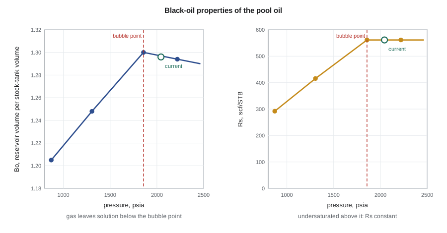
Reservoir hydrocarbons contain hundreds of chemical species, but most oil reservoirs can be described with only two hydrocarbon pseudo-components: the liquid that ends up in the stock tank and the gas that comes off at the separator. The black-oil model assumes that the reservoir oil phase contains stock-tank oil plus dissolved gas, that the reservoir gas phase contains only surface gas (or, in an extended model, also vaporized oil), and that water is a separate component that does not mix with the hydrocarbons. The split between phases depends only on pressure and is given by the same quantities that appear in a standard PVT report.
The oil formation volume factor B_o is the reservoir volume of oil per stock-tank volume, the solution gas-oil ratio R_s is the volume of surface gas dissolved per volume of stock-tank oil, B_g is the reservoir volume of free gas per surface volume and B_w is the water formation volume factor. With these, the three component equations of the black-oil model are written per unit bulk volume in surface volumes:
The gas equation has two parts because surface gas travels both as free gas and dissolved in the oil. The saturations sum to one, S_o + S_w + S_g = 1, and the phase pressures are linked by the oil-water and gas-oil capillary pressures. That gives three equations for three primary unknowns in each block, usually chosen as the oil pressure and two saturations. When a block is above its bubble point there is no free gas, and the simulator switches the third unknown to the solution gas-oil ratio or the bubble point pressure; this variable switching is one of the details that make black-oil codes more delicate than they look.
Rock compressibility and the pressure equation
Porosity changes slightly with pressure because the rock compresses as the pore pressure falls. Simulators usually represent this with a rock compressibility c_r, so that φ = φ_ref [1 + c_r (p − p_ref)], or with a table of pore volume multipliers. Combined with fluid compressibility, it produces the total compressibility c_t that controls how fast pressure responds to withdrawals.
For a single slightly compressible phase, the mass balance and Darcy's law combine into the diffusivity equation, the same equation that underlies well test analysis:
It is a parabolic equation: a disturbance at one point is felt everywhere immediately, but its effect decays with distance and grows with time. Its character explains several numerical features met later in the course. Because pressure responds across the whole reservoir at once, the pressure part of the system is best solved implicitly. Saturation, by contrast, moves with the flow at a finite speed, behaving more like a wave, and is the source of numerical dispersion and front smearing.
A block material balance
The smallest possible simulation model is one block with one well. Its mass balance says that the change in oil in the block over a time step equals the oil produced. For an undersaturated oil with total compressibility c_t, the pressure falls at a rate given by the reservoir withdrawal divided by the pore volume times compressibility. The code below applies this to a single block of the pool model and looks up the black-oil properties at each new pressure. After three months at a modest rate, the block pressure drops below the bubble point and free gas would begin to form, at which point a real simulator would switch variables and start tracking a gas saturation.
# Black-oil table lookup and the pressure change in one grid block
SI = False
# black-oil table: pressure (kPa), Bo (rm3/sm3), Rs (sm3/sm3), oil viscosity (mPa.s)
table = [(6000, 1.205, 52.0, 0.98), (9000, 1.248, 74.0, 0.86), (12800, 1.300, 100.0, 0.72),
         (15300, 1.294, 100.0, 0.74)]
def interp(p, col):
    for (p1, *a), (p2, *b) in zip(table, table[1:]):
        if p1 <= p <= p2:
            return a[col] + (b[col] - a[col]) * (p - p1) / (p2 - p1)
    raise ValueError("pressure outside table")
# one block: 400 m x 400 m x 6.5 m, porosity 0.14, total compressibility 1.5e-6 per kPa
V = 400 * 400 * 6.5 * 0.14            # pore volume, m3
ct = 1.5e-6                            # 1/kPa
p = 14090.0                            # kPa, current block pressure
qo = 5.0                               # sm3/d oil produced from the block, no injection
Bo = interp(p, 0)
dpdt = -qo * Bo / (V * ct)             # kPa per day, slightly compressible single phase
for days in (1, 30, 90):
    pn = p + dpdt * days
    note = "  (below bubble point: free gas forms)" if pn < 12800 else ""
    if SI:
        print(f"after {days:3d} d: block pressure {pn:8.0f} kPa, Bo {interp(pn, 0):.3f}, mu_o {interp(pn, 2):.2f} mPa.s{note}")
    else:
        print(f"after {days:3d} d: block pressure {pn * 0.145038:7.0f} psia, Bo {interp(pn, 0):.3f} rb/STB, mu_o {interp(pn, 2):.2f} cp{note}")
print(f"pressure falls {abs(dpdt):.1f} kPa per day" if SI else f"pressure falls {abs(dpdt) * 0.145038:.2f} psi per day")after 1 d: block pressure 2039 psia, Bo 1.297 rb/STB, mu_o 0.73 cp after 30 d: block pressure 1914 psia, Bo 1.299 rb/STB, mu_o 0.72 cp after 90 d: block pressure 1656 psia, Bo 1.281 rb/STB, mu_o 0.77 cp (below bubble point: free gas forms) pressure falls 4.31 psi per day
Two points from this small calculation carry over to every simulation. First, the properties are not constants: B_o and μ_o change with every pressure update, which is what makes the equations nonlinear. Second, the bubble point is a threshold. Above it, oil and rock compressibility are small and pressure falls quickly for a given withdrawal. Below it, gas comes out of solution, total compressibility rises sharply and the pressure decline slows, but the gas saturation that forms changes the relative permeabilities and the producing gas-oil ratio. The Mission Canyon waterflood pilot was started partly to keep the pool above the bubble point.
Beyond black oil
The black-oil model fails when the composition of the phases changes in ways that pressure alone cannot describe. In a gas condensate, liquid drops out near the well as pressure falls below the dew point, and its composition depends on the path. In miscible gas or carbon dioxide injection, the injected gas extracts intermediate components from the oil and develops miscibility over a transition zone. For these processes a compositional simulator writes one mass balance for each of n_c components, with the component split between oil and gas at each block given by flash calculations with a cubic equation of state such as Peng-Robinson. The fluid is typically lumped into six to fifteen pseudo-components to keep the cost manageable.
Thermal simulators add an energy balance, with heat carried by the flowing fluids, conducted through the rock and lost to the formations above and below. Viscosity, which for heavy oil and bitumen falls by orders of magnitude between reservoir temperature and steam temperature, becomes a strong function of temperature. These models are used for steam-assisted gravity drainage and cyclic steam stimulation in the oil sands and heavy oil fields. Their equations follow the same pattern as the black-oil ones: an accumulation term, a flux term and a source term for each conserved quantity.
| Model | Conserved quantities per block | Typical use |
|---|---|---|
| Single phase | One fluid mass | Pressure transients, gas storage screening |
| Black oil | Oil, gas and water components | Depletion, waterflood, immiscible gas |
| Compositional | n_c hydrocarbon components and water | Condensates, volatile oil, miscible and carbon dioxide injection |
| Thermal | Components plus energy | Steam and hot-water processes in heavy oil |
| Dual porosity | Each of the above in matrix and fractures | Naturally fractured carbonates and tight rocks |
Worked problem
Checking a black-oil accumulation term
A block has pore volume 65,400 rb, oil saturation 0.70 and B_o = 1.294 at its current pressure. How much stock-tank oil does it contain? If the pressure falls and B_o rises to 1.300 with no change in saturation, how much oil has been expelled from the block?
Show solution
- Stock-tank oil = V_p S_o / B_o = 65,400 × 0.70 / 1.294 = 35,378 STB.
- At the new pressure the block holds 65,400 × 0.70 / 1.300 = 35,215 STB.
- The difference is the oil expelled by expansion: about 163 STB. In a simulator this volume must appear as flow out of the block or as well production.
Answer: About 35,378 STB initially and about 163 STB expelled. The accumulation term is simply the change in V_p S_o / B_o over the time step.
Checking the equations with units
Lena's last piece of advice on the equations is to check their units term by term. Every term of the oil equation, written per unit bulk volume, must have units of stock-tank volume per bulk volume per time. The accumulation term divides a dimensionless quantity, φ S_o / B_o, by time. The flux term divides a velocity in reservoir volume per area per time by B_o and takes its divergence over a length. The source term is a stock-tank rate per bulk volume. When a term does not reduce to the same units as the others, a factor is missing, usually a formation volume factor, a conversion constant or a density. The same check applied to the input deck catches the most common data errors: tables entered in the wrong units, viscosities in pascal seconds rather than millipascal seconds or compressibilities per psi in a metric model. Simulators accept whatever numbers they are given, and a unit error in a single table can propagate through every block of the model without any warning in the run log.
Common mistakes
MistakeTreating formation volume factors and viscosities as constants.
InsteadThey change with pressure and must be updated with every iteration; this is a main source of nonlinearity.
MistakeForgetting the dissolved gas in the gas equation.
InsteadSurface gas travels both as free gas and in solution in the oil, so both fluxes appear.
MistakeUsing a black-oil model for a miscible gas flood.
InsteadWhen phase compositions change significantly, use a compositional model.
MistakeOmitting rock compressibility in an undersaturated reservoir.
InsteadAbove the bubble point, rock compressibility can be a large share of total compressibility.
Summary and key terms
- Every simulator solves a mass balance for each conserved quantity: accumulation plus net outflow equals the well source.
- Multiphase Darcy's law gives each phase velocity from permeability, relative permeability, viscosity and the potential gradient.
- The black-oil model uses oil, gas and water components and PVT tables of B_o, R_s, B_g and B_w versus pressure.
- Saturations sum to one and phase pressures are linked by capillary pressure, leaving three unknowns per block.
- The pressure equation behaves like diffusion and the saturation equations like waves, which shapes the numerical methods.
- Compositional and thermal models add more components or an energy balance but keep the same structure.
- Continuity equation
- The statement that mass accumulation in a volume equals net inflow plus sources.
- Relative permeability
- The fraction of absolute permeability a phase can use at a given saturation.
- Mobility
- Relative permeability divided by viscosity for a phase.
- Formation volume factor
- Reservoir volume of a phase per unit surface volume of the corresponding component.
- Solution gas-oil ratio
- Surface gas volume dissolved in a unit volume of stock-tank oil at reservoir conditions.
- Variable switching
- Changing the primary unknown in a block when a phase appears or disappears.
- Total compressibility
- The sum of rock compressibility and saturation-weighted fluid compressibilities.
Practice problems
Work each problem on paper first, then reveal the answer to check.
What three quantities are conserved in a black-oil model?
Show answer
Stock-tank oil, surface gas and water.
Why does the gas equation contain R_s?
Show answer
Because part of the surface gas travels dissolved in the oil phase.
What happens in a black-oil simulator when a block falls below its bubble point?
Show answer
Free gas appears, so the simulator switches from solution gas-oil ratio to gas saturation as a primary unknown.
Why is the pressure equation usually solved implicitly?
Show answer
It is diffusive, so pressure responds across the whole system at once; explicit methods would need tiny time steps.
Lesson quiz · 5 questions
Score 60% or more to complete this lesson.
Create a free account to save your progress, take quizzes and earn a certificate.