
NUC-350 · Lesson 11 of 12 · 19 min
Core design codes
Every reload begins with the start-up physics tests: measured critical boron, rod worths and temperature coefficients at zero power, then flux maps at power. Hana's job for the coming outage is to prepare the predictions that the measurements will be compared with. "The codes are only as good as their last comparison with the plant," Teodora says. "Our license depends on showing, cycle after cycle, that the methods predict what the reactor actually does, within known uncertainties."
The calculation chain
Core physics calculations follow a chain of codes, each with a specific job:
| Step | What it does | Output |
|---|---|---|
| Nuclear data processing | turns evaluated data files into cross section libraries for the codes | multigroup or continuous-energy libraries |
| Lattice code | solves transport in one assembly or bundle cell, many groups, with depletion and branches | tables of few-group homogenized constants, pin factors, discontinuity factors |
| Core simulator | solves for the whole core in two or a few groups, with depletion, feedback and control | k, power distribution, burnup, boron, rod positions, margins |
| Pin power reconstruction | combines nodal results with lattice form factors | pin powers and peaking factors |
| Transient and safety codes | solve kinetics coupled to thermal hydraulics for accidents | power and temperature histories for safety analysis |
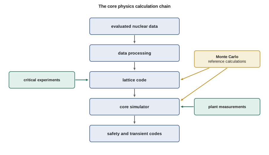
Nuclear data
Every calculation starts from evaluated nuclear data: the cross sections, fission yields, decay data and secondary particle distributions for every nuclide, compiled from measurements and nuclear models. Major libraries include ENDF/B from the United States, JEFF from the OECD Nuclear Energy Agency countries in Europe and JENDL from Japan. Processing codes such as NJOY convert these files into the forms that lattice and Monte Carlo codes use, including resonance data at each temperature. Changes from one library version to the next can shift calculated k by a few hundred pcm for some systems, so a methodology is always validated with a specific library.
Nodal core simulators
The core simulator solves the few-group diffusion equations, or a simplified transport approximation, for the whole three-dimensional core. Early codes used fine-mesh finite differences, which needed many mesh points per assembly. Modern codes use nodal methods, in which each node is typically one assembly wide, or a quarter of an assembly, and about 15 to 20 cm tall. Within each node, the flux is represented by polynomials or analytic functions, and the coupling between nodes is through the net currents across their faces. Nodal methods with discontinuity factors reach accuracy similar to fine-mesh solutions with far fewer unknowns, so a full core can be solved in seconds.
The simulator interpolates lattice constants for each node in the cross section table, using the node's burnup, fuel temperature, moderator density, boron or void, control state and history. It computes thermal hydraulic feedback with a simple channel model, depletes each node and tracks xenon and samarium. It also models the control system's actions, searching for the boron concentration or rod position that makes the core critical. For a reload design, the simulator runs the whole cycle in a few minutes and is repeated for thousands of cases during pattern optimization and safety evaluations.
The program below shows two pieces of this work in miniature: interpolating homogenized constants from a lattice table, as the simulator does for each node, and comparing predicted with measured critical boron and assembly powers, as the plant comparison does each cycle.
# Core design codes: the two-step method in miniature, and a code-versus-plant check.
# Step 1 (lattice code) tabulates homogenized constants against burnup.
# Step 2 (core simulator) interpolates them for each node. Values are illustrative.
table = {   # burnup MWd/kgU: (nu-Sigma_f thermal, Sigma_a thermal) for one assembly type
    0:  (0.1350, 0.0850), 10: (0.1240, 0.0830), 20: (0.1150, 0.0815),
    30: (0.1070, 0.0805), 40: (0.1000, 0.0798), 50: (0.0940, 0.0793)}
def lookup(bu):
    keys = sorted(table)
    for lo, hi in zip(keys, keys[1:]):
        if lo <= bu <= hi:
            w = (bu - lo) / (hi - lo)
            return tuple(table[lo][i] * (1 - w) + table[hi][i] * w for i in range(2))
    raise ValueError("burnup outside the table")
for bu in (5.0, 27.5, 44.0):
    nsf, sa = lookup(bu)
    print(f"node at {bu:4.1f} MWd/kgU: nu-Sigma_f = {nsf:.4f}, Sigma_a = {sa:.4f}, ratio = {nsf/sa:.3f}")
# Code-to-plant comparison: predicted versus measured critical boron (ppm) during a cycle
pred = [1450, 1210, 980, 760, 545, 330, 120]
meas = [1462, 1218, 995, 771, 551, 342, 131]
diff = [m - p for p, m in zip(pred, meas)]
mean = sum(diff) / len(diff)
sd = (sum((d - mean) ** 2 for d in diff) / (len(diff) - 1)) ** 0.5
print(f"critical boron, measured minus predicted: mean {mean:+.1f} ppm, standard deviation {sd:.1f} ppm")
# Flux map: predicted versus measured relative assembly powers at 8 monitored locations
p = [1.21, 1.08, 0.97, 1.30, 0.88, 1.15, 0.74, 1.02]
m = [1.23, 1.06, 0.96, 1.33, 0.87, 1.13, 0.76, 1.01]
rms = (sum(((mi - pi) / pi) ** 2 for pi, mi in zip(p, m)) / len(p)) ** 0.5
print(f"assembly power RMS difference: {rms * 100:.1f} %, largest {max(abs(mi - pi) / pi for pi, mi in zip(p, m)) * 100:.1f} %")node at 5.0 MWd/kgU: nu-Sigma_f = 0.1295, Sigma_a = 0.0840, ratio = 1.542 node at 27.5 MWd/kgU: nu-Sigma_f = 0.1090, Sigma_a = 0.0808, ratio = 1.350 node at 44.0 MWd/kgU: nu-Sigma_f = 0.0976, Sigma_a = 0.0796, ratio = 1.226 critical boron, measured minus predicted: mean +10.7 ppm, standard deviation 2.9 ppm assembly power RMS difference: 1.8 %, largest 2.7 %
The interpolated constants show the expected trend, with the ratio of production to absorption falling as burnup increases. The comparison with measurements gives a mean difference and a standard deviation, which together define the method's bias and uncertainty. In this example, the code predicts critical boron about 11 ppm low, consistently, with a small scatter. A consistent bias like this would be investigated and might be corrected in future predictions; the scatter feeds into the uncertainty allowance used in safety limits.
Uncertainties and safety limits
Safety limits are applied to calculated quantities with allowances for uncertainty. If the core simulator predicts a peak pin power, the true peak might be somewhat higher. The methodology therefore applies a factor, based on the statistical comparison of predictions with measurements, so that the limit is met with high confidence. For pin power peaking, typical allowances are a few percent. For reactivity quantities such as shutdown margin, allowances are given in pcm, and for rod worths as a percentage of the predicted worth.
Worked problem
An uncertainty allowance
A methodology's comparison with measured assembly powers gives a standard deviation of 1.8 percent. The allowance is set at about 1.645 standard deviations for one-sided 95 percent confidence. What multiplier is applied to predicted peak power?
Show solution
- Allowance = 1.645 × 1.8 % ≈ 3.0 %.
- Multiplier = 1.030.
Answer: A predicted peak of 1.45 becomes 1.49 when compared with the limit. In practice, the allowance also includes the uncertainty of the measurements themselves and a statistical tolerance for the number of comparisons.
Codes used for light-water reactor cores
In the U.S. industry, light-water reactor core design commonly uses lattice and core code systems from fuel vendors and commercial developers, such as the CASMO lattice code with the SIMULATE nodal simulator, and vendor-specific systems for pressurized and boiling water reactors. The U.S. Nuclear Regulatory Commission maintains its own codes for independent review, including PARCS for core neutronics and the SCALE system, which includes lattice and Monte Carlo capabilities. Utilities must use methods that the NRC has reviewed and approved in topical reports, and the technical specifications list the approved methods used to set the core operating limits for each cycle.
Verification, validation and quality assurance
Two words are used carefully. Verification asks whether the code solves its equations correctly: are the numerical methods implemented as intended, and do they converge to known analytic or highly accurate solutions? Validation asks whether the code, with its data and models, predicts reality: do its results agree with measurements and with trusted reference calculations? A code can be verified but not valid, if its models leave out important physics. Both are required, and both are documented.
Quality assurance surrounds the whole process. Code versions are controlled, so that a calculation can be repeated exactly years later. Input decks are checked by a second engineer. Changes to codes or data go through testing on a standard set of problems before release. Users are trained and qualified on the codes they run. This discipline may seem heavy, but it is what allows regulators, operators and the public to rely on calculated margins that cannot be measured directly.
Uncertainty quantification and new methods
Traditional methodologies give uncertainty allowances based on comparisons with measurements. Newer approaches add uncertainty quantification from first principles: propagating the uncertainties in nuclear data, manufacturing tolerances and models through the calculation chain, often by sampling, to estimate the uncertainty of each result. International benchmark projects compare these methods across codes and countries. Higher-fidelity methods, such as pin-resolved transport in the whole core and coupled multiphysics simulations, are moving from research into industrial use, first as references and then, as computers allow, for design. Machine learning is also being explored as a fast surrogate for core simulators in loading pattern optimization, always with final confirmation by the approved methods.
A week of plant comparisons
For a TVA reload, Hana's comparison follows a fixed routine. After start-up, she compares the measured critical boron at hot zero power, the measured worths of control banks and the measured isothermal temperature coefficient with the predictions she prepared. Once the unit is at power, she compares each flux map from the in-core detectors with the core simulator's predicted assembly powers, and follows the critical boron through the cycle. Any difference beyond the acceptance criteria is investigated: a measurement problem, an input error or a real difference in the core. The results feed the statistics that confirm the method's uncertainty allowances over time.
| Comparison | Typical frequency | What a large difference might indicate |
|---|---|---|
| Critical boron or reactivity balance | daily to monthly | error in burnable absorber modeling or depletion |
| Assembly or channel powers from in-core detectors | monthly flux maps or daily detector readings | loading error, detector fault or model bias |
| Rod or device worths | at start-up and after outages | error in lattice constants near devices |
| Temperature coefficients | at start-up | error in branch constants or feedback model |
These comparisons are more than a formality. Over many cycles they build a record of how well the methods predict each quantity, which is the evidence regulators review when methods are approved or changed. They also catch problems early: a small but growing difference in critical boron, for example, can reveal a modeling error in a new fuel design before it affects margins.
New codes and methods follow a careful path before they are used for licensing. A new version is first tested on a suite of verification problems with known answers, then on a validation set of critical experiments and plant cycles. Its results are compared with those of the version it replaces, and any differences are explained. Only when the methodology report has been reviewed, and approved where required, does the new version enter production. Experienced engineers often say that more effort goes into qualifying a code than into writing it.
Training matters as much as the codes themselves. A core physics engineer must know not only how to run a code but also what its approximations are and where it is likely to be least accurate. Hana's training plan includes running benchmark problems by hand and with the codes, reviewing past cycle comparisons and working alongside a qualified engineer before she signs calculations on her own. That understanding is what allows an engineer to recognize when a result does not make sense.
Hana's summary for the week is short: no differences outside the expected bands, one detector flagged for maintenance and a small, steady trend that she recommends watching. Teodora adds it to the record. Most weeks are like this, and that steadiness, built over years, is what gives confidence in the calculations used to set safety margins.
Common mistakes
MistakeA well-verified code is automatically valid.
InsteadVerification checks the numerics; validation compares with reality. Both are needed.
MistakeCalculated peaking factors can be compared directly with limits.
InsteadAn uncertainty allowance, based on comparison with measurements, must be added first.
MistakeAny code can be used for licensing if its results look reasonable.
InsteadLicensing calculations must use reviewed and approved methods with controlled versions.
Summary and key terms
- Core physics uses a chain: nuclear data, lattice code, core simulator, pin power reconstruction and transient codes.
- Nodal simulators solve the whole core quickly using lattice constants interpolated for each node.
- Comparisons with plant measurements give the bias and uncertainty of a methodology.
- Safety limits are applied with uncertainty allowances derived from those comparisons.
- Verification, validation and quality assurance are required for every code used in licensing.
- Evaluated nuclear data
- Recommended cross sections and other nuclear data compiled from experiments and models.
- Nodal method
- A core solution method using large nodes with polynomial or analytic flux shapes inside each.
- Core simulator
- A code that models the whole core in few groups, with depletion, feedback and control.
- Verification
- Showing that a code solves its equations correctly.
- Validation
- Showing that a code with its data and models predicts real behavior.
- Uncertainty allowance
- A margin added to calculated values to cover method and measurement uncertainty.
Practice problems
Work each problem on paper first, then reveal the answer to check.
What does the lattice code provide to the core simulator?
Show answer
Tables of few-group homogenized constants, pin form factors and discontinuity factors.
Why do nodal methods need fewer unknowns than fine-mesh methods?
Show answer
Each node is large, with a flux shape represented inside it, and discontinuity factors preserve accuracy.
In the example, what multiplier is applied for a 1.8 % standard deviation?
Show answer
About 1.030.
What is the difference between verification and validation?
Show answer
Verification checks that equations are solved correctly; validation checks agreement with reality.
Why must code versions be controlled?
Show answer
So that licensing calculations can be repeated exactly and changes are tested before use.
Lesson quiz · 5 questions
Score 60% or more to complete this lesson.
Create a free account to save your progress, take quizzes and earn a certificate.