The CAPM, beta and the cost of capital (WACC)

In MBA-501, the cohort compared Cedarline Outdoor's return on invested capital, which had fallen from 12.1 to 8.0 percent, with a weighted average cost of capital of 9 percent, and concluded that Cedarline's growth was destroying value. Grace asked at the time where the 9 percent came from, and Dr. Achterberg promised that this course would answer. Dr. Varga now does. The cost of capital is the return investors could expect elsewhere on investments of the same risk; it is an opportunity cost, set by markets, not a number a company chooses. Estimating it requires three steps: a measure of risk, a model linking risk to required return, and a way of combining the costs of the firm's different sources of money.

Beta: measuring systematic risk

Lesson 7 showed that only systematic risk is rewarded. Beta measures it. A share's beta is the sensitivity of its returns to the returns of the market as a whole: the covariance of the share's return with the market's, divided by the variance of the market's return. A beta of 1 means the share tends to move one for one with the market. A beta of 1.5 means that when the market rises or falls 10 percent, the share tends to rise or fall 15 percent. A beta of 0.5 means it tends to move half as much. The market itself has a beta of exactly 1, and the beta of a portfolio is the weighted average of the betas of its holdings.

In practice, beta is estimated by regressing a share's returns on the market's returns, typically using five years of monthly data or two years of weekly data. The slope of the regression is the beta. Estimates are noisy: a standard error of 0.2 or 0.3 is common for a single company, so a measured beta of 1.3 might plausibly be anywhere from 0.8 to 1.8. Analysts reduce the noise by averaging the betas of several comparable companies, and data providers often adjust raw estimates toward 1, because betas far from 1 tend to move back toward it over time.

# Estimating beta by regression on simulated monthly returns
import random, statistics as st
random.seed(511)
true_beta, months = 1.3, 60
market = [random.gauss(0.007, 0.045) for _ in range(months)]
share = [0.001 + true_beta * m + random.gauss(0, 0.06) for m in market]
mx, my = st.mean(market), st.mean(share)
cov = sum((x - mx) * (y - my) for x, y in zip(market, share)) / (months - 1)
beta = cov / st.variance(market)
resid = [y - (my + beta * (x - mx)) for x, y in zip(market, share)]
se = (sum(e * e for e in resid) / (months - 2)) ** 0.5 / (st.variance(market) * (months - 1)) ** 0.5
print(f"estimated beta {beta:.2f}, standard error {se:.2f}")
print(f"rough 95% range {beta - 2 * se:.2f} to {beta + 2 * se:.2f}")
print(f"adjusted beta (two thirds raw, one third 1.0): {2 / 3 * beta + 1 / 3:.2f}")

estimated beta 1.24, standard error 0.17
rough 95% range 0.90 to 1.58
adjusted beta (two thirds raw, one third 1.0): 1.16

The capital asset pricing model

The capital asset pricing model, developed in the 1960s by William Sharpe, John Lintner and others, says that in equilibrium the expected return on any asset equals the risk-free rate plus its beta times the market risk premium, the extra return investors expect for holding the market portfolio rather than risk-free assets.

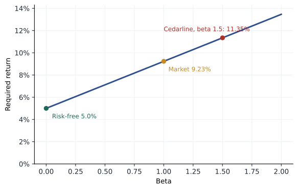
Plotted with beta on the horizontal axis and expected return on the vertical, the CAPM is a straight line, the security market line. Every asset, if fairly priced, should lie on it. An asset above the line offers more return than its systematic risk requires and is a bargain; one below is overpriced. For a company, the line gives the minimum return a project must earn: a project with a beta of 1.3 must be expected to earn at least the return on the line at 1.3.

Choosing the inputs

The risk-free rate should match the horizon of the cash flows being valued. For long-lived investments, practitioners usually use the yield on long-term government bonds, here the ten-year Treasury yield, close to 5.0 percent in late October 2026. The equity risk premium is the hardest input and the most debated. Historical averages of US equity returns over Treasury bonds since 1928 suggest about 5 points; forward-looking estimates infer the premium from current prices and expected cash flows. Aswath Damodaran of New York University, whose estimates are widely used, put the implied premium for the US market at 4.23 percent at the start of 2026, and surveys of corporate finance officers typically report premiums of 4 to 6 percent. Dr. Varga uses Damodaran's 4.23 percent in class, and stresses that a difference of a point in the premium changes the cost of equity by more than a point for a high-beta company.

The CAPM is a simplification. It assumes that investors care only about expected return and variance, can borrow and lend at the risk-free rate and agree on expectations. Empirical tests have found that the security market line is flatter than the model predicts, and that other characteristics, such as company size, value as measured by book-to-market ratios, and momentum, help explain average returns. Eugene Fama and Kenneth French developed multifactor models to capture these effects. Yet surveys show that most large companies still use the CAPM to estimate their cost of equity, because it is transparent, links required return to the kind of risk that cannot be diversified, and is hard to replace with something clearly better for decisions. Dr. Varga's advice is to use it with care, to test a range of inputs, and to cross-check against other methods, such as the implied cost of equity from the Gordon model in lesson 4.

The cost of debt

The cost of debt is the return lenders require today on new borrowing, not the coupon rate on old debt. For a company with traded bonds, it is the yield to maturity on those bonds. For a company without them, such as Northfield, it can be estimated from its bank borrowing rate or from the yields of bonds with the same credit rating. Because interest is deductible for tax purposes, the after-tax cost of debt is the pre-tax rate times one minus the tax rate. Lesson 9 discusses limits on that deduction.

Weighted average cost of capital

A company is funded by both debt and equity, so its overall cost of capital is the weighted average of the two, with weights equal to the market values of each source as a share of the total. This is the WACC, the discount rate applied to free cash flow to the firm in lesson 4.

The weights should be based on market values, not book values, because investors' required returns are on what their claims are worth today, and they should reflect the firm's target capital structure if it differs from today's mix. Cedarline is private, but the private equity investor's purchase of its stake two years ago valued the equity at about 300 million dollars, and its debt, including the lease liabilities that MBA-501 counted as debt, is about 190 million, so equity is about 61 percent of capital and debt 39 percent. Its equity beta, estimated from listed outdoor apparel companies and relevered at Cedarline's leverage with the method of lesson 9, is about 1.5.

# Cedarline Outdoor: cost of equity by CAPM and the WACC
rf, erp, beta = 0.050, 0.0423, 1.50     # 10-year government yield, equity risk premium, beta
kd, tax = 0.066, 0.25                   # pre-tax cost of debt, combined tax rate
equity_value, debt_value = 300.0, 190.0 # values, millions; debt includes leases
ke = rf + beta * erp
V = equity_value + debt_value
wacc = equity_value / V * ke + debt_value / V * kd * (1 - tax)
print(f"cost of equity {ke:.2%}, after-tax cost of debt {kd * (1 - tax):.2%}")
print(f"weights: equity {equity_value / V:.0%}, debt {debt_value / V:.0%}")
print(f"WACC {wacc:.2%}")

cost of equity 11.34%, after-tax cost of debt 4.95%
weights: equity 61%, debt 39%
WACC 8.87%

The result, about 9 percent, confirms the figure used in MBA-501. It also confirms the conclusion: Cedarline's return on invested capital of 8 percent falls short of what its investors require, so its recent expansion has been destroying value.

Project and divisional costs of capital

The WACC is the right discount rate only for projects with the same risk as the firm as a whole. Using a single company-wide rate for every project has a predictable consequence: risky projects look too good and safe ones too bad, so the firm drifts toward riskier investments and becomes riskier itself. Prairie Ridge's proposed dealership acquisition from lesson 7 should be evaluated at a cost of capital appropriate to farm equipment dealers, not to an energy producer.

The usual method is the pure-play approach. Find listed companies whose business resembles the project, estimate their betas, and remove the effect of their borrowing to get an asset beta, the beta the business would have with no debt. Then relever it at the capital structure planned for the project. Lesson 9 introduces the Hamada formula used for that adjustment. For Hana, whose not-for-profit has no shares, the same approach applies: the risk of a new outpatient clinic is best estimated from listed health care providers, adjusted for Lakeview's funding.

Dr. Varga also warns against two common errors. One is to add an arbitrary premium for risks that are diversifiable, such as the chance a specific product launch fails; those risks belong in the cash-flow forecasts, as scenarios with probabilities, not in the discount rate. The other is to use the firm's borrowing rate as the discount rate because a project is funded with a loan. The project's risk, not its funding source, determines its cost of capital.

For private companies such as Northfield, the same method applies with two adjustments. There is no share price, so beta must come from listed comparables, and the owners are often undiversified, which some practitioners address by adding a premium to the cost of equity. Dr. Varga prefers to estimate the market cost of capital first and to consider the owners' lack of diversification separately, because mixing the two hides an important judgment inside a single number.