σ-algebras and measures

Lesson 1 showed that we cannot assign a length to every subset of the line and keep the properties we want. The way out is to decide in advance which sets will be measured. This lesson sets up the abstract framework that the rest of the course uses: σ-algebras, which are the collections of measurable sets, and measures, which are countably additive functions on them. The framework is deliberately general. The same definitions describe length on the line, area in the plane, the number of elements of a set, and the probability of an event, and every theorem we prove about measures applies to all of them at once.

σ-algebras

Definition 2.1. Let \(X\) be a set. A collection \(\mathcal{A}\) of subsets of \(X\) is a σ-algebra if (i) \(X \in \mathcal{A}\); (ii) if \(E \in \mathcal{A}\), then its complement \(E^c = X \setminus E\) is in \(\mathcal{A}\); and (iii) if \(E_1, E_2, \ldots \in \mathcal{A}\), then \(\bigcup_{k=1}^{\infty} E_k \in \mathcal{A}\). The pair \((X, \mathcal{A})\) is a measurable space, and the members of \(\mathcal{A}\) are the measurable sets.

Several consequences follow immediately. The empty set is \(X^c\), so it is measurable. By De Morgan's law, \(\bigcap E_k = \big(\bigcup E_k^c\big)^c\), so countable intersections of measurable sets are measurable. Finite unions are included, since we may take \(E_k = \varnothing\) for large \(k\), and differences \(A \setminus B = A \cap B^c\) are measurable. In short, a σ-algebra is closed under all the set operations we can perform countably many times. The letter σ, as in the word series, signals the countable unions; a collection closed only under complements and finite unions is called an algebra.

Examples. The power set \(\mathcal{P}(X)\) of all subsets of \(X\) is the largest σ-algebra, and \(\{\varnothing, X\}\) is the smallest. On an uncountable set \(X\), the collection of sets that are countable or have countable complement is a σ-algebra: a countable union of countable sets is countable, and if some \(E_j\) has countable complement then so does the union. The collection of finite unions of intervals in \([0, 1]\) is an algebra but not a σ-algebra, since the countable union \(\bigcup_k \big[\frac{1}{2k+1}, \frac{1}{2k}\big]\) is not a finite union of intervals.

Generated σ-algebras and Borel sets

An intersection of any family of σ-algebras on \(X\), even an uncountable family, is again a σ-algebra: each of the three conditions holds in every member, so it holds in the intersection. Given any collection \(\mathcal{C}\) of subsets of \(X\), the σ-algebra generated by \(\mathcal{C}\), written \(\sigma(\mathcal{C})\), is the intersection of all σ-algebras containing \(\mathcal{C}\). There is at least one, the power set, so the definition makes sense. By construction \(\sigma(\mathcal{C})\) is the smallest σ-algebra containing \(\mathcal{C}\): any σ-algebra that contains \(\mathcal{C}\) contains \(\sigma(\mathcal{C})\).

Definition 2.2. The Borel σ-algebra \(\mathcal{B}(\mathbb{R})\) is the σ-algebra generated by the open subsets of \(\mathbb{R}\). Its members are the Borel sets. More generally, for any metric space or topological space, the Borel sets are those generated by the open sets.

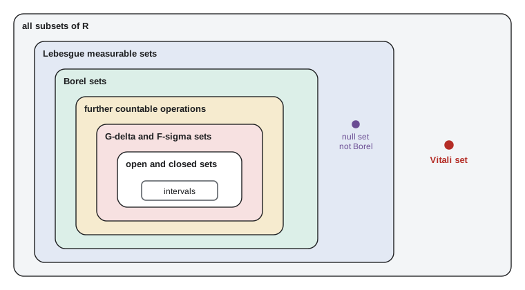
Every open and every closed set is Borel, and so are countable intersections of open sets, called \(G_\delta\) sets, and countable unions of closed sets, called \(F_\sigma\) sets. The rationals form an \(F_\sigma\) set, a countable union of points, and the irrationals a \(G_\delta\) set. Many different generating families give the same Borel σ-algebra. For instance, \(\mathcal{B}(\mathbb{R}) = \sigma(\{(a, b) : a < b\}) = \sigma(\{(-\infty, b] : b \in \mathbb{R}\})\). To prove the first equality, note that every open set is a countable union of open intervals with rational endpoints, so it lies in the σ-algebra generated by intervals; conversely, every open interval is open. For the second, \((a, b) = \bigcup_n (-\infty, b - \frac{1}{n}] \setminus (-\infty, a]\), and each half-line \((-\infty, b]\) is closed. The second description is the one used in probability, where a distribution is determined by its cumulative distribution function \(F(b) = P((-\infty, b])\).

Measures

Definition 2.3. A measure on a measurable space \((X, \mathcal{A})\) is a function \(\mu : \mathcal{A} \to [0, \infty]\) with \(\mu(\varnothing) = 0\) and countable additivity: if \(E_1, E_2, \ldots \in \mathcal{A}\) are pairwise disjoint, then \[\mu\Big(\bigcup_{k=1}^{\infty} E_k\Big) = \sum_{k=1}^{\infty} \mu(E_k).\] The triple \((X, \mathcal{A}, \mu)\) is a measure space. It is finite if \(\mu(X) < \infty\), a probability space if \(\mu(X) = 1\), and σ-finite if \(X\) is a countable union of measurable sets of finite measure.

The value \(\infty\) is allowed, with the conventions \(a + \infty = \infty\) for \(a \in [0, \infty]\) and that a series of nonnegative terms always has a sum in \([0, \infty]\). This makes the definition clean: the right side of countable additivity always has a meaning, regardless of the order of the terms.

Examples. Counting measure on any set \(X\), with \(\mathcal{A} = \mathcal{P}(X)\), assigns to \(E\) the number of its elements, or \(\infty\) if \(E\) is infinite. The Dirac measure at a point \(x_0\) assigns \(\delta_{x_0}(E) = 1\) if \(x_0 \in E\) and \(0\) otherwise; it models a unit mass concentrated at one point. On a countable set with weights \(w_x \ge 0\), \(\mu(E) = \sum_{x \in E} w_x\) is a measure, and when the weights sum to \(1\) it is a discrete probability distribution. On the σ-algebra of countable and co-countable subsets of an uncountable set, the function equal to \(0\) on countable sets and \(1\) on co-countable sets is a measure. Lebesgue measure on the Borel sets, which gives each interval its length, will be constructed in lesson 3; for now we take its existence on trust and use it in examples.

Basic properties

Theorem 2.4. Let \((X, \mathcal{A}, \mu)\) be a measure space and let all sets below be measurable. (a) Monotonicity: if \(A \subseteq B\) then \(\mu(A) \le \mu(B)\). (b) Countable subadditivity: \(\mu\big(\bigcup_k E_k\big) \le \sum_k \mu(E_k)\) for any sequence, disjoint or not. (c) Continuity from below: if \(E_1 \subseteq E_2 \subseteq \cdots\), then \(\mu\big(\bigcup_k E_k\big) = \lim_k \mu(E_k)\). (d) Continuity from above: if \(E_1 \supseteq E_2 \supseteq \cdots\) and \(\mu(E_1) < \infty\), then \(\mu\big(\bigcap_k E_k\big) = \lim_k \mu(E_k)\).

Proof. (a) Write \(B = A \cup (B \setminus A)\), a disjoint union, so \(\mu(B) = \mu(A) + \mu(B \setminus A) \ge \mu(A)\). (b) Disjointify: let \(F_1 = E_1\) and \(F_k = E_k \setminus \bigcup_{j<k} E_j\). The \(F_k\) are measurable, pairwise disjoint, satisfy \(F_k \subseteq E_k\), and have the same union as the \(E_k\). Hence \(\mu\big(\bigcup E_k\big) = \sum \mu(F_k) \le \sum \mu(E_k)\) by (a). (c) With the same disjointification, now \(F_k = E_k \setminus E_{k-1}\) (with \(E_0 = \varnothing\)) and \(E_n = F_1 \cup \cdots \cup F_n\). Thus \[\mu\Big(\bigcup_k E_k\Big) = \sum_{k=1}^{\infty} \mu(F_k) = \lim_{n \to \infty} \sum_{k=1}^{n} \mu(F_k) = \lim_{n \to \infty} \mu(E_n).\] (d) The sets \(E_1 \setminus E_k\) increase to \(E_1 \setminus \bigcap_k E_k\). By (c), \(\mu(E_1) - \mu\big(\bigcap E_k\big) = \lim_k \big(\mu(E_1) - \mu(E_k)\big)\), where we used finiteness of \(\mu(E_1)\) to subtract. Rearranging gives the result. \(\blacksquare\)

The finiteness assumption in (d) cannot be dropped. With counting measure on \(\mathbb{N}\), the sets \(E_k = \{k, k+1, k+2, \ldots\}\) decrease to the empty set, but \(\mu(E_k) = \infty\) for every \(k\). Similarly, for Lebesgue measure the half-lines \([k, \infty)\) decrease to \(\varnothing\) while each has infinite length. Continuity from above is the first place where infinite measure behaves differently, and we will meet the same phenomenon in the convergence theorems.

Null sets and completeness

A set \(N \in \mathcal{A}\) with \(\mu(N) = 0\) is a null set. A property that holds at every point outside a null set is said to hold almost everywhere, abbreviated a.e., or almost surely in probability. For example, the Dirichlet function equals zero almost everywhere with respect to Lebesgue measure. Countable unions of null sets are null by subadditivity, so countably many almost-everywhere statements can be combined into one: if each \(P_k\) holds a.e., then all of them hold simultaneously a.e.

A subset of a null set need not be measurable. A measure space is complete if every subset of a null set is measurable (and hence null by monotonicity). Lebesgue measure on the Borel σ-algebra is not complete, as we will see in lesson 4, but every measure space has a completion: the σ-algebra \(\overline{\mathcal{A}} = \{E \cup Z : E \in \mathcal{A}, Z \subseteq N \text{ for some null } N\}\) with \(\overline{\mu}(E \cup Z) = \mu(E)\). Checking that this is a σ-algebra, that \(\overline{\mu}\) is well defined, and that it is a complete measure extending \(\mu\) is a good exercise in the definitions. The completion of Borel measure is exactly the Lebesgue measure produced by Carathéodory's construction in lesson 3.

Uniqueness: the π–λ theorem

When do two measures agree? If they agree on a generating family, must they agree on the whole σ-algebra? Not in general, but they do if the family is closed under intersections and the measures are finite. A family \(\mathcal{P}\) is a π-system if \(A, B \in \mathcal{P}\) implies \(A \cap B \in \mathcal{P}\). A family \(\mathcal{L}\) is a λ-system, or Dynkin system, if it contains \(X\), is closed under proper differences \(B \setminus A\) for \(A \subseteq B\), and is closed under increasing unions. Eugene Dynkin's π–λ theorem states that if a π-system \(\mathcal{P}\) is contained in a λ-system \(\mathcal{L}\), then \(\sigma(\mathcal{P}) \subseteq \mathcal{L}\).

Corollary 2.5. If two finite measures \(\mu, \nu\) with \(\mu(X) = \nu(X)\) agree on a π-system \(\mathcal{P}\), they agree on \(\sigma(\mathcal{P})\). Proof: the collection \(\mathcal{L}\) of sets where \(\mu = \nu\) contains \(X\), is closed under proper differences because \(\mu(B \setminus A) = \mu(B) - \mu(A)\) for finite measures, and is closed under increasing unions by continuity from below. It is a λ-system containing \(\mathcal{P}\), so it contains \(\sigma(\mathcal{P})\). \(\blacksquare\) Applied to half-lines \((-\infty, b]\), which form a π-system generating the Borel sets, the corollary says that a probability distribution on the line is determined by its distribution function. The same argument, applied on each piece of a σ-finite decomposition, shows that Lebesgue measure is the only measure on the Borel sets that gives every interval its length.

Computing with finite σ-algebras

On a finite set every σ-algebra is generated by a partition into atoms, the minimal nonempty measurable sets, and every measurable set is a union of atoms. A σ-algebra with \(k\) atoms therefore has exactly \(2^k\) members. This is the model case for the idea that a σ-algebra represents information: in probability, knowing which atom of a σ-algebra contains the outcome is knowing everything the σ-algebra can distinguish. The code generates the σ-algebra spanned by a few subsets by closing under complements and unions, and reads off its atoms.

# Generate the sigma-algebra on a finite set from a few subsets, and find its atoms.
from itertools import combinations

X = frozenset(range(1, 9))
gens = [frozenset({1, 2, 3}), frozenset({3, 4, 5, 6})]

def generate(X, gens):
    S = {frozenset(), X} | set(gens)
    while True:
        new = {X - A for A in S} | {A | B for A, B in combinations(S, 2)}
        if new <= S:
            return S
        S |= new

S = generate(X, gens)
atoms = sorted((A for A in S if A and not any(B and B < A for B in S)), key=min)
print("number of measurable sets:", len(S))
print("atoms:", [sorted(a) for a in atoms])
print("2 ** (number of atoms) =", 2 ** len(atoms))

# a measure is determined by its values on the atoms
weights = {1: 0.1, 2: 0.1, 3: 0.2, 4: 0.05, 5: 0.15, 6: 0.1, 7: 0.2, 8: 0.1}
mu = lambda A: round(sum(weights[x] for x in A), 10)
print("mu of each atom:", [mu(a) for a in atoms])
print("additivity check:", mu(atoms[0] | atoms[2]), "=", round(mu(atoms[0]) + mu(atoms[2]), 10))

number of measurable sets: 16
atoms: [[1, 2], [3], [4, 5, 6], [7, 8]]
2 ** (number of atoms) = 16
mu of each atom: [0.2, 0.2, 0.3, 0.3]
additivity check: 0.5 = 0.5

For infinite sets nothing so simple is true. The Borel σ-algebra has no atoms other than points, and it cannot be built by finitely many closure steps. One can show that it has the cardinality of the continuum, while the power set of \(\mathbb{R}\) is strictly larger, so most subsets of the line are not Borel. Yet every set we can describe explicitly by countable operations on intervals is Borel, which is why the Borel σ-algebra is large enough for analysis.

A practical consequence for the rest of the course is the generating-family principle: to prove that every set in \(\sigma(\mathcal{C})\) has some property, show that the sets with the property form a σ-algebra (or a λ-system, with \(\mathcal{C}\) a π-system) containing \(\mathcal{C}\). We have already used it twice, for the Borel generators and for uniqueness of measures, and we will use it again for measurable functions and for product measures.