Product measures and the theorems of Fubini and Tonelli

Computing an area by integrating the lengths of its cross-sections, or a double integral as an iterated one, is so familiar from calculus that it is easy to forget it needs a proof. In measure theory the question becomes: given measure spaces \((X, \mathcal{A}, \mu)\) and \((Y, \mathcal{B}, \nu)\), is there a measure on \(X \times Y\) that assigns to each rectangle \(A \times B\) the product \(\mu(A)\nu(B)\), and when is the integral of a function with respect to it equal to either iterated integral? The answers are the product measure construction and two theorems: Tonelli's, which allows iteration for every nonnegative measurable function, and Fubini's, which allows it for every integrable function. Both require σ-finiteness, and we will see examples showing that neither hypothesis can be dropped.

The product σ-algebra

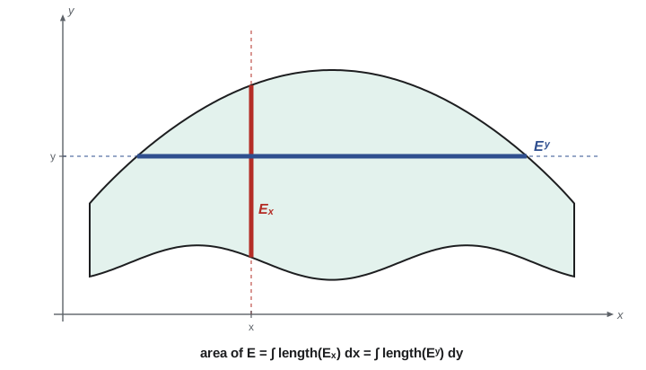
A measurable rectangle is a set \(A \times B\) with \(A \in \mathcal{A}\) and \(B \in \mathcal{B}\). The product σ-algebra \(\mathcal{A} \otimes \mathcal{B}\) is the σ-algebra on \(X \times Y\) generated by the measurable rectangles. For \(E \subseteq X \times Y\), the sections are \[E_x = \{y \in Y : (x, y) \in E\}, \qquad E^y = \{x \in X : (x, y) \in E\}.\] For a function \(f\) on \(X \times Y\), the sections are \(f_x(y) = f(x, y)\) and \(f^y(x) = f(x, y)\).

Proposition 10.1. If \(E \in \mathcal{A} \otimes \mathcal{B}\), then \(E_x \in \mathcal{B}\) for every \(x\) and \(E^y \in \mathcal{A}\) for every \(y\). If \(f\) is \(\mathcal{A} \otimes \mathcal{B}\)-measurable, every section \(f_x\) is \(\mathcal{B}\)-measurable and every \(f^y\) is \(\mathcal{A}\)-measurable.

Proof. The collection of sets \(E \subseteq X \times Y\) all of whose \(x\)-sections are in \(\mathcal{B}\) is a σ-algebra, because taking sections commutes with complements and countable unions: \((E^c)_x = (E_x)^c\) and \(\big(\bigcup E_k\big)_x = \bigcup (E_k)_x\). It contains every rectangle, since \((A \times B)_x\) is \(B\) or \(\varnothing\). So it contains \(\mathcal{A} \otimes \mathcal{B}\). For functions, \(\{f_x > a\} = \{f > a\}_x\). \(\blacksquare\)

For the Borel sets, \(\mathcal{B}(\mathbb{R}) \otimes \mathcal{B}(\mathbb{R}) = \mathcal{B}(\mathbb{R}^2)\): every open subset of the plane is a countable union of open rectangles with rational corners, and conversely every rectangle with Borel sides is Borel in the plane. For the Lebesgue σ-algebra \(\mathcal{L}\), however, \(\mathcal{L} \otimes \mathcal{L}\) is strictly smaller than the Lebesgue σ-algebra of the plane: if \(V\) is a Vitali set, \(\{0\} \times V\) is a subset of a null line, hence Lebesgue measurable in the plane, but its section at \(x = 0\) is \(V\), so it is not in \(\mathcal{L} \otimes \mathcal{L}\).

Constructing the product measure

Theorem 10.2. Let \(\mu\) and \(\nu\) be σ-finite. For every \(E \in \mathcal{A} \otimes \mathcal{B}\), the functions \(x \mapsto \nu(E_x)\) and \(y \mapsto \mu(E^y)\) are measurable, and \[\int_X \nu(E_x) \, d\mu(x) = \int_Y \mu(E^y) \, d\nu(y).\] The common value \((\mu \times \nu)(E)\) defines a measure on \(\mathcal{A} \otimes \mathcal{B}\), the unique measure with \((\mu \times \nu)(A \times B) = \mu(A)\nu(B)\) for all measurable rectangles.

Proof. First assume \(\mu\) and \(\nu\) finite. Let \(\mathcal{L}\) be the collection of \(E \in \mathcal{A} \otimes \mathcal{B}\) for which both functions are measurable and the two integrals agree. For a rectangle, \(\nu((A \times B)_x) = \nu(B)\mathbf{1}_A(x)\), and both integrals equal \(\mu(A)\nu(B)\), so rectangles are in \(\mathcal{L}\); they form a π-system, since \((A \times B) \cap (A^\prime \times B^\prime) = (A \cap A^\prime) \times (B \cap B^\prime)\). The collection \(\mathcal{L}\) contains \(X \times Y\). It is closed under proper differences: if \(E \subseteq F\) are in \(\mathcal{L}\), then \(\nu((F \setminus E)_x) = \nu(F_x) - \nu(E_x)\), a difference of measurable functions with finite integrals, and the integrals subtract. It is closed under increasing unions by the monotone convergence theorem, since \(\nu((E_k)_x) \uparrow \nu(E_x)\) by continuity from below. So \(\mathcal{L}\) is a λ-system containing the rectangles, and by the π–λ theorem it contains \(\mathcal{A} \otimes \mathcal{B}\).

In the σ-finite case write \(X = \bigcup X_j\) and \(Y = \bigcup Y_k\), increasing unions of sets of finite measure, and apply the finite case to the restrictions to \(X_j \times Y_k\). For \(E \in \mathcal{A} \otimes \mathcal{B}\), the sets \(E \cap (X_j \times Y_j)\) increase to \(E\), and monotone convergence carries measurability and equality of the integrals to the limit. Countable additivity of \(E \mapsto \int \nu(E_x) \, d\mu\) follows from Corollary 6.9, since \(\nu\big((\bigcup E_k)_x\big) = \sum_k \nu((E_k)_x)\) for disjoint \(E_k\). Uniqueness follows from the π–λ argument of lesson 2 on each \(X_j \times Y_j\). \(\blacksquare\)

Lebesgue measure on \(\mathbb{R}^2\) is the completion of \(m \times m\). The construction extends to finitely many factors, and \(m \times \cdots \times m\) on \(\mathbb{R}^n\), completed, is \(n\)-dimensional Lebesgue measure. The formula \((\mu \times \nu)(E) = \int \nu(E_x) \, d\mu\) is Cavalieri's principle: two solids whose cross-sections have equal areas at every height have equal volumes.

Tonelli and Fubini

Theorem 10.3 (Tonelli, 1909). Let \(\mu, \nu\) be σ-finite and \(f : X \times Y \to [0, \infty]\) be \(\mathcal{A} \otimes \mathcal{B}\)-measurable. Then \(x \mapsto \int_Y f(x, y) \, d\nu(y)\) and \(y \mapsto \int_X f(x, y) \, d\mu(x)\) are measurable, and \[\int_{X \times Y} f \, d(\mu \times \nu) = \int_X \Big( \int_Y f(x, y) \, d\nu(y) \Big) d\mu(x) = \int_Y \Big( \int_X f(x, y) \, d\mu(x) \Big) d\nu(y).\]

Proof. For \(f = \mathbf{1}_E\), this is Theorem 10.2. By linearity it holds for nonnegative simple functions. For general \(f \ge 0\), take simple \(\varphi_n \uparrow f\). For each \(x\), \((\varphi_n)_x \uparrow f_x\), so by monotone convergence \(\int \varphi_n(x, y) \, d\nu(y) \uparrow \int f(x, y) \, d\nu(y)\). These are increasing limits of measurable functions of \(x\), so they are measurable, and a second application of monotone convergence in \(x\), together with monotone convergence on \(X \times Y\), gives the result. \(\blacksquare\)

Theorem 10.4 (Fubini, 1907). Let \(\mu, \nu\) be σ-finite and \(f \in L^1(\mu \times \nu)\). Then \(f_x \in L^1(\nu)\) for almost every \(x\), \(f^y \in L^1(\mu)\) for almost every \(y\), the almost everywhere defined functions \(x \mapsto \int f_x \, d\nu\) and \(y \mapsto \int f^y \, d\mu\) are integrable, and the iterated integrals both equal \(\int f \, d(\mu \times \nu)\).

Proof. Apply Tonelli to \(|f|\): \(\int_X \big(\int_Y |f(x, y)| \, d\nu\big) d\mu = \int |f| < \infty\), so the inner integral is finite for almost every \(x\), that is, \(f_x \in L^1(\nu)\) a.e. Apply Tonelli separately to \(f^+\) and \(f^-\), each with finite integral, and subtract; the subtraction is legitimate on the full-measure set where both inner integrals are finite. \(\blacksquare\)

In practice the two theorems are used together: to justify exchanging the order of integration for a function of both signs, first compute an iterated integral of \(|f|\), which Tonelli allows in either order; if it is finite, Fubini applies. Guido Fubini proved his theorem in 1907, Leonida Tonelli the nonnegative version in 1909, and the measure-theoretic form for general σ-finite spaces came later. The theorems are often quoted together as the Fubini–Tonelli theorem.

Counterexamples

Without integrability the iterated integrals can differ. On \(\mathbb{N} \times \mathbb{N}\) with counting measure, let \(a_{m,n} = 1\) if \(m = n\), \(a_{m,n} = -1\) if \(n = m + 1\), and \(0\) otherwise. Each row \(m\) contains one \(1\) and one \(-1\), so every row sums to \(0\) and the sum of row sums is \(0\). Column \(1\) contains only the \(1\) at \((1, 1)\), and every later column contains one \(1\) and one \(-1\), so the sum of column sums is \(1\). The function is not integrable, since \(\sum |a_{m,n}| = \infty\).

A continuous example on \([0, 1]^2\) is \(f(x, y) = \frac{x^2 - y^2}{(x^2 + y^2)^2}\), with the origin excluded. Since \(\frac{\partial}{\partial y} \frac{y}{x^2 + y^2} = \frac{x^2 - y^2}{(x^2 + y^2)^2}\), the inner integral is \(\int_0^1 f(x, y) \, dy = \frac{1}{1 + x^2}\), and then \(\int_0^1 \frac{dx}{1 + x^2} = \frac{\pi}{4}\). By antisymmetry, integrating in the other order gives \(-\frac{\pi}{4}\). Again \(\int |f| = \infty\), because near the origin \(|f|\) behaves like \(\frac{1}{r^2}\) in polar coordinates, and \(\int_0^1 \frac{1}{r^2} r \, dr\) diverges.

Without σ-finiteness Tonelli can fail even for indicator functions. Let \(\mu\) be Lebesgue measure on \([0, 1]\), \(\nu\) counting measure on \([0, 1]\) (with the Borel sets), and \(D = \{(x, x)\}\) the diagonal, a closed set. Then \(\nu(D_x) = 1\) for each \(x\), so \(\int \nu(D_x) \, d\mu = 1\), while \(\mu(D^y) = 0\) for each \(y\), so \(\int \mu(D^y) \, d\nu = 0\). Counting measure on an uncountable set is not σ-finite, and no product measure with the rectangle property can be defined consistently. Wacław Sierpiński showed in 1920, assuming the continuum hypothesis, that there is a subset of the square, not product measurable, whose iterated integrals are both defined and different, which explains why the measurability hypothesis appears in both theorems.

# Iterated sums and integrals that disagree when the integrability hypothesis fails.
N = 400
a = lambda m, n: 1 if m == n else (-1 if n == m + 1 else 0)
row_sums = sum(sum(a(m, n) for n in range(1, N + 2)) for m in range(1, N + 1))
col_sums = sum(sum(a(m, n) for m in range(1, N + 2)) for n in range(1, N + 1))
print("sum of row sums:", row_sums, "  sum of column sums:", col_sums)

import math
def inner_dy(x, n=4000):
    """Midpoint rule for the integral over y in [0, 1] of (x^2 - y^2)/(x^2 + y^2)^2."""
    h = 1 / n
    return h * sum((x * x - y * y) / (x * x + y * y) ** 2 for y in ((j + 0.5) * h for j in range(n)))
xs = [(i + 0.5) / 400 for i in range(400)]
dy_first = sum(inner_dy(x) for x in xs) / 400
print(f"integrate dy then dx: {dy_first:.4f}   (exact pi/4 = {math.pi / 4:.4f})")
print(f"inner integral at x = 0.5: {inner_dy(0.5):.5f}   exact 1/(1 + x^2) = {1 / 1.25:.5f}")
print("integrate dx then dy: -pi/4 by antisymmetry, f(y, x) = -f(x, y)")

# Tonelli in action: the layer-cake formula  integral of f = integral over t of m({f > t}) dt
f = lambda x: x * x                  # on [0, 1]; m({x^2 > t}) = 1 - sqrt(t)
layer = sum(1 - math.sqrt((k + 0.5) / 2000) for k in range(2000)) / 2000
print(f"layer cake for x^2 on [0, 1]: {layer:.5f}   direct integral 1/3 = {1 / 3:.5f}")

sum of row sums: 0   sum of column sums: 1
integrate dy then dx: 0.7854   (exact pi/4 = 0.7854)
inner integral at x = 0.5: 0.80000   exact 1/(1 + x^2) = 0.80000
integrate dx then dy: -pi/4 by antisymmetry, f(y, x) = -f(x, y)
layer cake for x^2 on [0, 1]: 0.33333   direct integral 1/3 = 0.33333

Applications

The layer-cake formula. For measurable \(f \ge 0\) on a σ-finite space, \[\int_X f \, d\mu = \int_0^\infty \mu(\{f > t\}) \, dt.\] Proof: \(f(x) = \int_0^\infty \mathbf{1}_{\{t < f(x)\}} \, dt\). The set \(\{(x, t) : t < f(x)\}\) is product measurable, being the region under the graph, so Tonelli lets us exchange the integrals. This formula, which says that the area under a graph can be computed by horizontal slices, is the Lebesgue sum of lesson 1 in its exact form. In probability it reads \(E[X] = \int_0^\infty P(X > t) \, dt\) for \(X \ge 0\).

Convolution. For \(f, g \in L^1(\mathbb{R})\), the convolution \((f * g)(x) = \int f(x - y) g(y) \, dy\) is defined for almost every \(x\), and \(\|f * g\|_1 \le \|f\|_1 \|g\|_1\). Proof: the function \((x, y) \mapsto f(x - y)g(y)\) is measurable on the plane, and by Tonelli and translation invariance, \(\int \int |f(x - y)| |g(y)| \, dx \, dy = \int |g(y)| \big(\int |f(x - y)| \, dx\big) dy = \|f\|_1 \|g\|_1\). Fubini then shows that \(f * g\) is integrable, with \(\int f * g = \int f \int g\). In probability, if independent random variables have densities \(f\) and \(g\), their sum has density \(f * g\).

Independence. If \((X, \mathcal{A}, \mu)\) and \((Y, \mathcal{B}, \nu)\) are probability spaces, the product \(\mu \times \nu\) is the joint distribution of an independent pair. The factorization \(E[\varphi(X)\psi(Y)] = E[\varphi(X)] \, E[\psi(Y)]\) for integrable \(\varphi(X), \psi(Y)\) is Fubini's theorem applied to the product function. Kolmogorov's extension theorem builds product measures on infinitely many factors, which is how sequences of independent random variables, such as those in the laws of large numbers, are constructed.