Continuity in metric spaces and Arzelà–Ascoli (overview)

With open sets, convergence, completeness and compactness defined in any metric space, continuity comes next. The epsilon–delta definition from Real Analysis I carries over word for word, and so do its main consequences: continuous functions on compact spaces are bounded, attain their extreme values and are uniformly continuous. This lesson proves these facts in general, gives examples of continuous maps between spaces of functions, and then describes the compact subsets of \(C[a, b]\) by the Arzelà–Ascoli theorem.

Three equivalent definitions

Definition. Let \((X, d)\) and \((Y, \rho)\) be metric spaces. A map \(f: X \to Y\) is continuous at \(a \in X\) if for every \(\varepsilon > 0\) there is \(\delta > 0\) such that \(d(x, a) < \delta\) implies \(\rho(f(x), f(a)) < \varepsilon\). It is continuous if it is continuous at every point.

Equivalently, for every \(\varepsilon > 0\) there is \(\delta > 0\) with \(f(B(a, \delta)) \subseteq B(f(a), \varepsilon)\): every ball around \(f(a)\) contains the image of some ball around \(a\).

Theorem 9.1. For \(f: X \to Y\) the following are equivalent.

• (a) \(f\) is continuous.

• (b) Sequential continuity: whenever \(x_n \to x\) in \(X\), \(f(x_n) \to f(x)\) in \(Y\).

• (c) For every open \(V \subseteq Y\), the preimage \(f^{-1}(V) = \{x \in X : f(x) \in V\}\) is open in \(X\).

Proof. (a) implies (b): let \(x_n \to x\) and \(\varepsilon > 0\). Choose \(\delta\) for continuity at \(x\), and \(N\) with \(d(x_n, x) < \delta\) for \(n \ge N\). Then \(\rho(f(x_n), f(x)) < \varepsilon\) for \(n \ge N\).

(b) implies (a): suppose \(f\) is not continuous at \(a\). Then for some \(\varepsilon > 0\) no \(\delta\) works, so for each \(n\) there is \(x_n\) with \(d(x_n, a) < \frac{1}{n}\) but \(\rho(f(x_n), f(a)) \ge \varepsilon\). Then \(x_n \to a\) while \(f(x_n) \not\to f(a)\), contradicting (b).

(a) implies (c): let \(V\) be open and \(a \in f^{-1}(V)\). Since \(f(a) \in V\) and \(V\) is open, some \(B(f(a), \varepsilon) \subseteq V\). Continuity gives \(\delta\) with \(f(B(a, \delta)) \subseteq B(f(a), \varepsilon) \subseteq V\), so \(B(a, \delta) \subseteq f^{-1}(V)\). Hence \(f^{-1}(V)\) is open.

(c) implies (a): given \(a\) and \(\varepsilon\), the ball \(V = B(f(a), \varepsilon)\) is open, so \(f^{-1}(V)\) is an open set containing \(a\). It contains some \(B(a, \delta)\), which means \(f(B(a, \delta)) \subseteq V\). \(\square\)

Taking complements, (c) is equivalent to: preimages of closed sets are closed. Characterization (c) is how continuity is defined in a general topological space, where there are open sets but no distances, and it is the starting point of MATH-447. It makes some facts immediate. The composition of continuous maps is continuous, since \((g \circ f)^{-1}(W) = f^{-1}(g^{-1}(W))\). And sets defined by strict inequalities between continuous functions are open: \(\{(x, y) \in \mathbb{R}^2 : x^2 + y^3 < 1\}\) is the preimage of the open set \((-\infty, 1)\) under a continuous function.

Examples of continuous maps

Definition. A map \(f: X \to Y\) is Lipschitz with constant \(L\) if \(\rho(f(x), f(y)) \le L\,d(x, y)\) for all \(x, y\). A Lipschitz map is continuous, indeed uniformly continuous: take \(\delta = \frac{\varepsilon}{L}\).

• The distance to a fixed point, \(x \mapsto d(x, a)\), is Lipschitz with constant 1 from \(X\) to \(\mathbb{R}\), by the reverse triangle inequality.

• A linear map \(A: \mathbb{R}^n \to \mathbb{R}^m\) with matrix \((a_{ij})\) is Lipschitz. By Cauchy–Schwarz each coordinate satisfies \(|(Ax)_i| \le \sqrt{\sum_j a_{ij}^2}\,|x|\), so \(|Ax| \le \sqrt{\sum_{i,j} a_{ij}^2}\,|x|\) in the Euclidean norm, and \(|Ax - Ay| = |A(x - y)|\).

• On \(C[a, b]\) with the sup metric, evaluation at a point, \(f \mapsto f(c)\), is Lipschitz with constant 1, since \(|f(c) - g(c)| \le d_\infty(f, g)\).

• On \(C[a, b]\) with the sup metric, integration \(f \mapsto \int_a^b f\) is Lipschitz with constant \(b - a\). This is theorem 3.3, restated as continuity of a map on a metric space.

• On \(C[a, b]\), the map \(f \mapsto \max f\) is Lipschitz with constant 1. If \(\max f = f(c)\), then \(\max f - \max g \le f(c) - g(c) \le d_\infty(f, g)\), and symmetrically.

Not every natural map on a function space is continuous. On the space of continuously differentiable functions on \([0, 1]\) with the sup metric, \(f \mapsto f^\prime(0)\) is not continuous at 0: \(f_n(x) = \frac{\sin(n^2x)}{n}\) satisfies \(d_\infty(f_n, 0) \le \frac{1}{n}\) but \(f_n^\prime(0) = n\). This is lesson 3's failure of term-by-term differentiation, seen as discontinuity of differentiation.

Continuity and compactness

Theorem 9.2. If \(K\) is compact and \(f: K \to Y\) is continuous, then \(f(K)\) is compact.

Proof. Let \(\{V_\alpha\}\) be an open cover of \(f(K)\). By theorem 9.1 each \(f^{-1}(V_\alpha)\) is open, and these sets cover \(K\). By compactness finitely many, \(f^{-1}(V_{\alpha_1}), \dots, f^{-1}(V_{\alpha_m})\), cover \(K\), and then \(V_{\alpha_1}, \dots, V_{\alpha_m}\) cover \(f(K)\). \(\square\)

Corollary 9.3 (extreme value theorem). A continuous function \(f: K \to \mathbb{R}\) on a nonempty compact metric space is bounded and attains its maximum and minimum.

Proof. \(f(K)\) is a compact subset of \(\mathbb{R}\), so closed and bounded by theorem 8.6. Its supremum is a limit of points of \(f(K)\), so it belongs to the closed set \(f(K)\); that is, it is a value \(f(c)\). Similarly for the infimum. \(\square\)

Theorem 9.4 (Heine–Cantor). A continuous map from a compact metric space \(K\) to a metric space \(Y\) is uniformly continuous: for every \(\varepsilon > 0\) there is \(\delta > 0\) such that \(d(x, y) < \delta\) implies \(\rho(f(x), f(y)) < \varepsilon\), for all \(x, y \in K\).

Proof. If not, there are \(\varepsilon > 0\) and points \(x_n, y_n\) with \(d(x_n, y_n) < \frac{1}{n}\) and \(\rho(f(x_n), f(y_n)) \ge \varepsilon\). By sequential compactness a subsequence \(x_{n_k}\) converges to some \(p \in K\), and then \(y_{n_k} \to p\) too, since \(d(y_{n_k}, p) \le d(y_{n_k}, x_{n_k}) + d(x_{n_k}, p)\). By continuity at \(p\), both \(f(x_{n_k})\) and \(f(y_{n_k})\) tend to \(f(p)\), so \(\rho(f(x_{n_k}), f(y_{n_k})) \to 0\), a contradiction. \(\square\)

Equicontinuity

The Heine–Borel theorem describes the compact subsets of \(\mathbb{R}^n\). In \(C[a, b]\) closed and bounded sets need not be compact, as the disjoint tents of lesson 8 showed: they are uniformly bounded, but they become steeper and steeper. The missing ingredient is a uniform control on oscillation across the whole family.

Definition. A family \(\mathcal{F}\) of functions on \([a, b]\) is equicontinuous if for every \(\varepsilon > 0\) there is \(\delta > 0\) such that \(|f(x) - f(y)| < \varepsilon\) for all \(f \in \mathcal{F}\) and all \(x, y \in [a, b]\) with \(|x - y| < \delta\). It is uniformly bounded if there is \(M\) with \(|f(x)| \le M\) for all \(f \in \mathcal{F}\) and all \(x\).

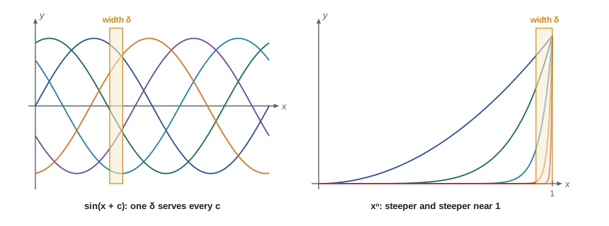
Each single continuous function on \([a, b]\) is uniformly continuous by Heine–Cantor; equicontinuity asks for one \(\delta\) that serves every member of the family. A family of differentiable functions with a common bound \(|f^\prime| \le L\) is equicontinuous, by the mean value theorem: \(|f(x) - f(y)| \le L|x - y|\), so \(\delta = \frac{\varepsilon}{L}\) works for all of them. The family \(\{\sin(x + c) : c \in \mathbb{R}\}\) is equicontinuous. The families \(\{x^n\}\) on \([0, 1]\) and \(\{\sin(nx)\}\) on \([0, \pi]\) are not: in each, for every \(\delta > 0\) some member changes by at least \(\frac{1}{2}\) over an interval of length less than \(\delta\).

import math

def modulus(funcs, a, b, delta):
    """Estimate sup over the family and over |x - y| <= delta of |f(x) - f(y)| on a grid."""
    h, step = delta / 4, 4                      # four grid steps per window of width delta
    pts = int((b - a) / h) + 1
    worst = 0.0
    for f in funcs:
        v = [f(a + i * h) for i in range(pts)]
        for i in range(pts - step):
            worst = max(worst, abs(v[i + step] - v[i]))
    return worst

families = [
    ("sin(x + c), c = 0..49", [lambda x, c=c: math.sin(x + c) for c in range(50)], 0, 2 * math.pi),
    ("x^n, n = 1..50 on [0,1]", [lambda x, n=n: x ** n for n in range(1, 51)], 0, 1),
    ("sin(nx), n = 1..50 on [0,pi]", [lambda x, n=n: math.sin(n * x) for n in range(1, 51)], 0, math.pi),
    ("sin(nx)/n, n = 1..50", [lambda x, n=n: math.sin(n * x) / n for n in range(1, 51)], 0, math.pi),
]
print("family                          delta=0.1   delta=0.01   delta=0.001")
for name, fs, a, b in families:
    row = [modulus(fs, a, b, d) for d in (0.1, 0.01, 0.001)]
    print(f"{name:<30}" + "".join(f"{r:12.4f}" for r in row))

family                          delta=0.1   delta=0.01   delta=0.001
sin(x + c), c = 0..49               0.1000      0.0100      0.0010
x^n, n = 1..50 on [0,1]             0.9948      0.3950      0.0488
sin(nx), n = 1..50 on [0,pi]        1.9993      0.4948      0.0500
sin(nx)/n, n = 1..50                0.0998      0.0100      0.0010

For the translates of \(\sin\) and for \(\frac{\sin(nx)}{n}\), whose derivatives are all bounded by 1, the worst change over a window of width \(\delta\) is about \(\delta\), so it shrinks with \(\delta\). For \(x^n\) and \(\sin(nx)\) with \(n\) up to 50 it shrinks too, but only once \(\delta\) is smaller than about \(\frac{1}{50}\): enlarging the family to all \(n\) would keep the worst change near 1 for \(x^n\), and near 2 for \(\sin(nx)\), for every \(\delta\), which is exactly the failure of equicontinuity. A finite family is always equicontinuous; the question is what happens as the family grows.

The Arzelà–Ascoli theorem

Theorem 9.5 (Arzelà–Ascoli). Let \((f_n)\) be a sequence in \(C[a, b]\) that is uniformly bounded and equicontinuous. Then \((f_n)\) has a subsequence that converges uniformly on \([a, b]\). Conversely, if every sequence in a family \(\mathcal{F} \subseteq C[a, b]\) has a uniformly convergent subsequence, then \(\mathcal{F}\) is uniformly bounded and equicontinuous.

Proof of the first part. List the rational numbers in \([a, b]\) as \(q_1, q_2, \dots\). The real sequence \((f_n(q_1))\) is bounded, so by Bolzano–Weierstrass it has a convergent subsequence; call that subsequence of functions \(f_{1,1}, f_{1,2}, \dots\). The values of these functions at \(q_2\) are bounded, so a further subsequence \(f_{2,1}, f_{2,2}, \dots\) converges at \(q_2\), and still at \(q_1\). Continuing, the \(j\)-th sequence converges at \(q_1, \dots, q_j\). The diagonal sequence \(g_k = f_{k,k}\) is a subsequence of \((f_n)\), and from the \(j\)-th term on it is a subsequence of the \(j\)-th sequence, so \((g_k(q_j))\) converges for every \(j\).

We show \((g_k)\) is uniformly Cauchy. Let \(\varepsilon > 0\) and take \(\delta\) from equicontinuity. Finitely many of the rationals, say \(r_1, \dots, r_m\), have the property that every \(x \in [a, b]\) is within \(\delta\) of one of them, since the rationals are dense and \([a, b]\) is covered by finitely many intervals of length \(\delta\). Choose \(K\) with \(|g_k(r_i) - g_l(r_i)| < \varepsilon\) for all \(k, l \ge K\) and \(i = 1, \dots, m\). For any \(x\), pick \(r_i\) with \(|x - r_i| < \delta\). Then for \(k, l \ge K\), \[|g_k(x) - g_l(x)| \le |g_k(x) - g_k(r_i)| + |g_k(r_i) - g_l(r_i)| + |g_l(r_i) - g_l(x)| < 3\varepsilon.\] So \((g_k)\) is uniformly Cauchy, and it converges uniformly by theorem 2.2. \(\square\)

Proof of the converse. If \(\mathcal{F}\) is not uniformly bounded, choose \(f_n \in \mathcal{F}\) with \(\|f_n\|_\infty > n\); a uniformly convergent subsequence would have bounded sup norms, as uniform limits of bounded functions are bounded, so none exists. If \(\mathcal{F}\) is not equicontinuous, there are \(\varepsilon > 0\), \(f_n \in \mathcal{F}\) and \(x_n, y_n\) with \(|x_n - y_n| < \frac{1}{n}\) and \(|f_n(x_n) - f_n(y_n)| \ge \varepsilon\). If a subsequence \(f_{n_k}\) converged uniformly to \(f\), then \(f\) would be continuous, hence uniformly continuous, and \(|f_{n_k}(x_{n_k}) - f_{n_k}(y_{n_k})| \le 2\|f_{n_k} - f\|_\infty + |f(x_{n_k}) - f(y_{n_k})| \to 0\), a contradiction. \(\square\)

In the language of lesson 8, a closed subset of \(C[a, b]\) is compact if and only if it is uniformly bounded and equicontinuous: the Heine–Borel theorem for spaces of continuous functions. The diagonal argument used in the proof, extracting a subsequence of a subsequence of a subsequence and then taking the diagonal, is one of the most useful tricks in analysis.

Giulio Ascoli introduced equicontinuity in a paper of 1883–84 and proved that it gives the sufficient condition; Cesare Arzelà, who had worked with the idea since the early 1880s, established the necessary condition and gave the first clear general statement in 1895. The theorem was soon put to work. Giuseppe Peano's existence theorem of 1890 says that \(y^\prime = F(x, y)\), \(y(x_0) = y_0\), has a solution near \(x_0\) whenever \(F\) is merely continuous; its modern proof builds approximate solutions by Euler's method, which are equicontinuous because their slopes are bounded by \(\max |F|\), and extracts a convergent subsequence by Arzelà–Ascoli. Without a Lipschitz condition the solution need not be unique, so the contraction mapping theorem cannot be used. A full treatment, and the generalization to compact metric spaces, belongs to functional analysis.