Capstone: the implicit function theorem and applications

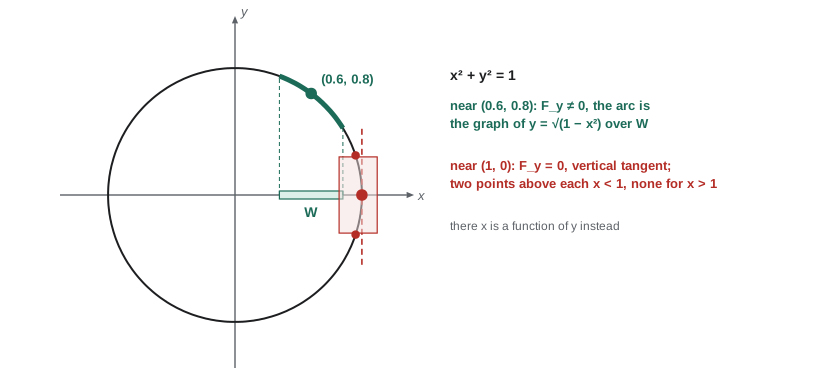
The equation \(x^2 + y^2 = 1\) does not define \(y\) as a function of \(x\): each \(x\) in \((-1, 1)\) has two partners \(\pm\sqrt{1 - x^2}\). Yet near any point of the circle other than \((\pm 1, 0)\), the circle is the graph of a single differentiable function, one of the two square roots. The implicit function theorem says when an equation, or a system of equations, can be solved locally for some of the variables as differentiable functions of the others, and it gives the derivatives of the solution without solving. This capstone lesson proves it from the inverse function theorem, applies it to curves, surfaces and Lagrange multipliers, and draws together the threads of the course.

The statement

Write points of \(\mathbb{R}^{n+m}\) as \((x, y)\) with \(x \in \mathbb{R}^n\) and \(y \in \mathbb{R}^m\). For a \(C^1\) map \(F: U \to \mathbb{R}^m\) on an open set \(U \subseteq \mathbb{R}^{n+m}\), split the Jacobian into the \(m \times n\) block \(D_xF\) of partial derivatives in the \(x\) variables and the square \(m \times m\) block \(D_yF\) of partial derivatives in the \(y\) variables, so that \(DF = (D_xF \ \ D_yF)\).

Theorem 12.1 (implicit function theorem). Let \(F: U \to \mathbb{R}^m\) be continuously differentiable on an open set \(U \subseteq \mathbb{R}^{n+m}\), and let \((a, b) \in U\) satisfy \(F(a, b) = 0\) with \(D_yF(a, b)\) invertible. Then there are an open set \(\Omega \subseteq U\) containing \((a, b)\), an open set \(W \subseteq \mathbb{R}^n\) containing \(a\), and a \(C^1\) map \(g: W \to \mathbb{R}^m\) with \(g(a) = b\), such that a point \((x, y) \in \Omega\) satisfies \(F(x, y) = 0\) if and only if \(x \in W\) and \(y = g(x)\). Moreover \[Dg(x) = -D_yF(x, g(x))^{-1}\,D_xF(x, g(x)) \quad \text{for } x \in W.\]

So near \((a, b)\), the solution set of the \(m\) equations \(F = 0\) in \(n + m\) unknowns is the graph of a \(C^1\) function of \(n\) of the variables. The hypothesis says that the linearized equations \(D_xF\,u + D_yF\,v = 0\) can be solved uniquely for \(v\) in terms of \(u\), and the conclusion says the same for the nonlinear equations, locally. As with the inverse function theorem, the linear approximation decides.

The proof

Proof. Define \(\Phi: U \to \mathbb{R}^{n+m}\) by \(\Phi(x, y) = (x, F(x, y))\). It is \(C^1\), and its Jacobian has the block form \[D\Phi = \begin{pmatrix} I & 0 \\ D_xF & D_yF \end{pmatrix},\] whose determinant is \(\det D_yF\). At \((a, b)\) this is nonzero, so by the inverse function theorem there are open sets \(\Omega \ni (a, b)\) and \(V \ni \Phi(a, b) = (a, 0)\) such that \(\Phi\) maps \(\Omega\) one-to-one onto \(V\) with \(C^1\) inverse \(\Psi: V \to \Omega\).

Since \(\Phi\) does not change the first coordinate, neither does \(\Psi\): \(\Psi(x, z) = (x, h(x, z))\) for a \(C^1\) map \(h\). Let \(W = \{x \in \mathbb{R}^n : (x, 0) \in V\}\). It is open, as the preimage of the open set \(V\) under the continuous map \(x \mapsto (x, 0)\), and it contains \(a\). Define \(g(x) = h(x, 0)\) for \(x \in W\); it is \(C^1\), and \(g(a) = b\) because \(\Psi(a, 0) = (a, b)\).

For \(x \in W\), \(\Phi(x, g(x)) = \Phi(\Psi(x, 0)) = (x, 0)\), so \((x, g(x)) \in \Omega\) and \(F(x, g(x)) = 0\). Conversely, if \((x, y) \in \Omega\) and \(F(x, y) = 0\), then \(\Phi(x, y) = (x, 0) \in V\), so \(x \in W\), and \(\Phi(x, y) = \Phi(x, g(x))\) with both points in \(\Omega\), where \(\Phi\) is one-to-one; hence \(y = g(x)\).

For the derivative, \(D\Phi\) is invertible on \(\Omega\), since \(D\Phi\,D\Psi = I\) by the chain rule, so \(\det D_yF \ne 0\) at every point of \(\Omega\). Differentiating the identity \(F(x, g(x)) = 0\) with the chain rule gives \(D_xF(x, g(x)) + D_yF(x, g(x))\,Dg(x) = 0\), and solving for \(Dg(x)\) gives the formula. \(\square\)

The derivative formula is often used on its own, under the name implicit differentiation. For one equation \(F(x, y) = 0\) in two variables it reads \(g^\prime(x) = -\frac{F_x}{F_y}\), which is the rule taught in a first calculus course. The theorem supplies what that course takes for granted: that a differentiable solution \(y = g(x)\) exists in the first place.

Curves in the plane

The code checks the derivative formula numerically. For each \(x\) near \(\frac{3}{2}\) it computes \(g(x)\) by Newton's method in the single unknown \(y\), started from the known solution, and then compares a central difference of \(g\) with \(-\frac{F_x}{F_y}\).

import math

F  = lambda x, y: x ** 3 + y ** 3 - 3 * x * y
Fx = lambda x, y: 3 * x * x - 3 * y
Fy = lambda x, y: 3 * y * y - 3 * x

def g(x, y0=1.5):
    """Solve F(x, y) = 0 for y near y0 by Newton's method in y."""
    y = y0
    for _ in range(50):
        step = F(x, y) / Fy(x, y)
        y -= step
        if abs(step) < 1e-15:
            break
    return y

t = 1e-5
print("    x       g(x)          slope by differences   -Fx/Fy")
for x in [1.2, 1.3, 1.4, 1.5, 1.55]:
    y = g(x)
    numeric = (g(x + t) - g(x - t)) / (2 * t)
    formula = -Fx(x, y) / Fy(x, y)
    print(f"{x:5.2f}   {y:.10f}    {numeric:14.8f}       {formula:11.8f}")
print("residual F(1.55, g(1.55)) =", F(1.55, g(1.55)))

    x       g(x)          slope by differences   -Fx/Fy
 1.20   1.5840140801        0.11000994        0.11000994
 1.30   1.5857206871       -0.08586122       -0.08586122
 1.40   1.5637149640       -0.37914594       -0.37914594
 1.50   1.5000000000       -1.00000000       -1.00000000
 1.55   1.4309524533       -1.95236917       -1.95236915
residual F(1.55, g(1.55)) = 0.0

The two slope columns agree to about seven decimal places, and at \(x = 1.5\) the slope is exactly \(-1\), as computed by hand. Newton's method converges at each \(x\) because the starting value 1.5 is close to the solution and \(F_y\) stays away from 0 along this part of the curve. The range of \(x\) cannot be pushed much further: the loop of the folium reaches only to \(x = 2^{2/3} \approx 1.587\), where its tangent is vertical and \(F_y = 0\), and beyond that this branch has no points at all. The theorem guarantees a solution only on some neighborhood, and this one is not large.

Systems and surfaces

With more equations the same theorem describes curves and surfaces in space. One equation \(G(x, y, z) = 0\) with \(\nabla G \ne 0\) at a point defines, near that point, a surface that is the graph of a \(C^1\) function of two of the variables: if \(G_z \ne 0\), it is \(z = g(x, y)\) with \(g_x = -\frac{G_x}{G_z}\) and \(g_y = -\frac{G_y}{G_z}\). Two equations define a curve.

This is the beginning of the theory of manifolds. A subset of \(\mathbb{R}^{n+m}\) that is locally the solution set of \(m\) equations with linearly independent gradients is a smooth manifold of dimension \(n\), and the implicit function theorem says that near each of its points it looks like the graph of a function on an open subset of \(\mathbb{R}^n\). Spheres, tori and the group of rotations of space all arise this way, and MATH-430 develops their geometry.

Lagrange multipliers

Theorem 12.2 (Lagrange multipliers). Let \(f, G: U \to \mathbb{R}\) be \(C^1\) on an open set \(U \subseteq \mathbb{R}^n\), let \(M = \{x \in U : G(x) = 0\}\), and let \(p \in M\) with \(\nabla G(p) \ne 0\). If the restriction of \(f\) to \(M\) has a local maximum or minimum at \(p\), then there is a number \(\lambda\) with \[\nabla f(p) = \lambda\,\nabla G(p).\]

Proof. Since \(\nabla G(p) \ne 0\), some partial derivative is nonzero; renumbering the variables, \(\frac{\partial G}{\partial x_n}(p) \ne 0\). Write \(x = (x^\prime, x_n)\) with \(x^\prime \in \mathbb{R}^{n-1}\) and \(p = (p^\prime, p_n)\). By the implicit function theorem there are an open \(W \ni p^\prime\) and a \(C^1\) function \(g\) on \(W\) with \(g(p^\prime) = p_n\) such that, near \(p\), the points of \(M\) are exactly the points \((x^\prime, g(x^\prime))\), and \(\frac{\partial g}{\partial x_j} = -\frac{\partial_jG}{\partial_nG}\) along this graph. The function \(\phi(x^\prime) = f(x^\prime, g(x^\prime))\) then has a local extremum at the interior point \(p^\prime\) of \(W\), so all its partial derivatives vanish there. By the chain rule, for \(j < n\), \[0 = \frac{\partial \phi}{\partial x_j}(p^\prime) = \partial_jf(p) + \partial_nf(p)\frac{\partial g}{\partial x_j}(p^\prime) = \partial_jf(p) - \partial_nf(p)\frac{\partial_jG(p)}{\partial_nG(p)}.\] Put \(\lambda = \frac{\partial_nf(p)}{\partial_nG(p)}\). Then \(\partial_jf(p) = \lambda\,\partial_jG(p)\) for \(j < n\), and for \(j = n\) this holds by the definition of \(\lambda\). \(\square\)

Joseph-Louis Lagrange introduced the multipliers in his Mécanique analytique of 1788, to handle constraints in mechanics, long before a rigorous implicit function theorem existed. Geometrically, at a constrained extremum the gradient of \(f\) has no component along the constraint surface, so it must be perpendicular to the surface, that is, parallel to \(\nabla G\). The condition is necessary, not sufficient, and it fails without the hypothesis \(\nabla G(p) \ne 0\): on the cusp \(G(x, y) = y^2 - x^3 = 0\), the function \(f = x\) is minimized at the origin, where \(\nabla f = (1, 0)\) but \(\nabla G = (0, 0)\).

As a bonus computation, the code finds the maximum of \(f(x, y) = xy\) on the ellipse \(x^2 + 4y^2 = 8\) by solving the Lagrange system \(\nabla f = \lambda\nabla G\), \(G = 0\), three equations in \(x, y, \lambda\), with Newton's method in \(\mathbb{R}^3\). By hand: \(y = 2\lambda x\) and \(x = 8\lambda y\) give \(\lambda = \pm\frac{1}{4}\); with \(\lambda = \frac{1}{4}\), \(y = \frac{x}{2}\) and \(2x^2 = 8\), so the maximum is \(f(2, 1) = 2\).

def system(v):
    x, y, lam = v
    return [y - lam * 2 * x,             # f_x - lam G_x, with f = xy, G = x^2 + 4y^2 - 8
            x - lam * 8 * y,             # f_y - lam G_y
            x * x + 4 * y * y - 8]       # G = 0

def jac(v):
    x, y, lam = v
    return [[-2 * lam, 1, -2 * x],
            [1, -8 * lam, -8 * y],
            [2 * x, 8 * y, 0]]

def solve3(A, b):
    """Gaussian elimination with partial pivoting for a 3 by 3 system."""
    M = [row[:] + [bi] for row, bi in zip(A, b)]
    for c in range(3):
        piv = max(range(c, 3), key=lambda r: abs(M[r][c]))
        M[c], M[piv] = M[piv], M[c]
        for r in range(c + 1, 3):
            m = M[r][c] / M[c][c]
            M[r] = [a - m * p for a, p in zip(M[r], M[c])]
    x = [0.0] * 3
    for r in (2, 1, 0):
        x[r] = (M[r][3] - sum(M[r][k] * x[k] for k in range(r + 1, 3))) / M[r][r]
    return x

v = [1.5, 1.2, 0.3]                       # rough guess
for k in range(8):
    step = solve3(jac(v), [-s for s in system(v)])
    v = [a + s for a, s in zip(v, step)]
    res = max(abs(s) for s in system(v))
    print(f"step {k + 1}: x = {v[0]:.12f}  y = {v[1]:.12f}  lambda = {v[2]:.12f}  residual = {res:.1e}")
print("maximum of xy on the ellipse:", round(v[0] * v[1], 12))

step 1: x = 1.999821556031  y = 1.042764097074  lambda = 0.247623721152  residual = 3.5e-01
step 2: x = 2.001099940496  y = 1.000349519898  lambda = 0.249951401975  residual = 7.2e-03
step 3: x = 2.000000192746  y = 1.000000115849  lambda = 0.249999978158  residual = 1.7e-06
step 4: x = 2.000000000000  y = 1.000000000000  lambda = 0.250000000000  residual = 9.1e-14
step 5: x = 2.000000000000  y = 1.000000000000  lambda = 0.250000000000  residual = 0.0e+00
step 6: x = 2.000000000000  y = 1.000000000000  lambda = 0.250000000000  residual = 0.0e+00
step 7: x = 2.000000000000  y = 1.000000000000  lambda = 0.250000000000  residual = 0.0e+00
step 8: x = 2.000000000000  y = 1.000000000000  lambda = 0.250000000000  residual = 0.0e+00
maximum of xy on the ellipse: 2.0

More applications

Smooth dependence of roots. A simple root of a polynomial depends smoothly on the coefficients. For example \(F(t, x) = x^3 + tx - 1\) has the root \(x = 1\) at \(t = 0\), and \(F_x = 3x^2 + t = 3 \ne 0\) there, so for \(t\) near 0 there is a unique root \(x(t)\) near 1, depending smoothly on \(t\), with \(x^\prime(0) = -\frac{F_t}{F_x} = -\frac{x}{3x^2 + t} = -\frac{1}{3}\). At a double root, where \(F_x = 0\), roots can collide and disappear, as for \(x^2 + t = 0\), which has two real roots for \(t < 0\) and none for \(t > 0\).

Comparative statics. In economics, equilibrium conditions \(F(x, y) = 0\) relate endogenous variables \(y\), such as prices, to exogenous parameters \(x\), such as taxes. The implicit function theorem shows that when \(D_yF\) is invertible, the equilibrium responds smoothly to small changes in the parameters, and its formula gives the response \(Dg = -D_yF^{-1}D_xF\) without solving the model.

Thermodynamics. If three quantities are linked by one equation \(F(p, V, T) = 0\), such as an equation of state, and all three partial derivatives of \(F\) are nonzero, each quantity is locally a function of the other two, and the theorem gives \(\frac{\partial p}{\partial V} = -\frac{F_V}{F_p}\), \(\frac{\partial V}{\partial T} = -\frac{F_T}{F_V}\) and \(\frac{\partial T}{\partial p} = -\frac{F_p}{F_T}\). Multiplying, \[\frac{\partial p}{\partial V}\,\frac{\partial V}{\partial T}\,\frac{\partial T}{\partial p} = -1,\] the triple product rule, whose minus sign surprises anyone who treats partial derivatives as fractions. For an ideal gas \(pV = nRT\) it can be checked directly.

Looking back

The course began with a failure: pointwise limits of continuous functions can be discontinuous, as Abel's example showed in 1826. Uniform convergence, which Weierstrass made central, repaired continuity and integration, and with uniform convergence of derivatives also differentiation. The M-test made uniform convergence easy to verify for series, power series turned out to converge uniformly inside their intervals, and Weierstrass's approximation theorem showed that polynomials are dense among continuous functions.

Uniform convergence is convergence in the sup metric, and that observation led to metric spaces. Completeness of \(C[a, b]\) in the sup metric, compactness and its failure in infinite dimensions, and the Arzelà–Ascoli theorem form the basic toolkit of analysis on spaces of functions. Completeness also gave the contraction mapping theorem, which solved integral equations and then, combined with the derivative as a linear map, proved the inverse and implicit function theorems. Every major theorem of the second half rests on the completeness of the real numbers established in MATH-241.

The next steps branch. MATH-441 replaces the Riemann integral by the Lebesgue integral, whose convergence theorems handle limits of integrals with far weaker hypotheses than uniform convergence. MATH-447 abstracts open sets into general topology. MATH-430 uses the implicit function theorem to study curves, surfaces and manifolds. And functional analysis treats spaces such as \(C[a, b]\) as infinite-dimensional analogues of \(\mathbb{R}^n\), where the contraction mapping theorem, Arzelà–Ascoli and the inverse function theorem all reappear.