Power series and analytic functions on the real line

A power series centered at \(c\) is a series \(\sum_{k=0}^{\infty} a_k(x - c)^k\). Polynomials are the simplest functions there are, and power series are the next simplest: they can be added, multiplied, differentiated and integrated term by term inside their interval of convergence. This lesson proves those facts using the M-test, introduces analytic functions, and proves Abel's theorem on the behavior of a power series at the edge of its interval of convergence. To keep notation simple we take \(c = 0\); the general case follows by substituting \(x - c\) for \(x\).

The radius of convergence

Lemma 5.1. If \(\sum a_k x_0^k\) converges for some \(x_0 \ne 0\), then \(\sum a_k x^k\) converges absolutely for every \(x\) with \(|x| < |x_0|\).

Proof. The terms of a convergent series tend to 0, so they are bounded: \(|a_k x_0^k| \le C\) for all \(k\). For \(|x| < |x_0|\) put \(q = \frac{|x|}{|x_0|} < 1\). Then \(|a_k x^k| = |a_k x_0^k| q^k \le Cq^k\), and \(\sum Cq^k\) converges. By comparison, \(\sum |a_k x^k|\) converges. \(\square\)

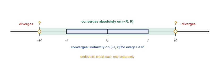
It follows that the set of points where the series converges is an interval centered at 0. Let \(R\) be the supremum of the \(|x|\) at which the series converges, with \(R = \infty\) if the set is unbounded. Then the series converges absolutely for \(|x| < R\) and diverges for \(|x| > R\). The number \(R\) is the radius of convergence. At the endpoints \(x = \pm R\) anything can happen: \(\sum x^k\) diverges at both, \(\sum \frac{x^k}{k}\) converges at \(-1\) but not at 1, and \(\sum \frac{x^k}{k^2}\) converges at both.

Theorem 5.2 (Cauchy–Hadamard). Let \(L = \limsup_{k \to \infty} |a_k|^{1/k}\), the largest limit of a subsequence of \(|a_k|^{1/k}\), or \(\infty\) if that sequence is unbounded. Then \(R = \frac{1}{L}\), with the conventions \(\frac{1}{0} = \infty\) and \(\frac{1}{\infty} = 0\). If \(\lim \big|\frac{a_{k+1}}{a_k}\big|\) exists, it also equals \(L\).

Proof. Apply the root test to \(\sum |a_k x^k|\): \(\limsup |a_k x^k|^{1/k} = L|x|\). If \(L|x| < 1\) the series converges absolutely, and if \(L|x| > 1\) the terms do not tend to 0, since \(|a_k x^k| > 1\) for infinitely many \(k\), so it diverges. Hence \(R = \frac{1}{L}\). The ratio statement follows from the ratio test in the same way. \(\square\)

Augustin-Louis Cauchy stated the formula in his Cours d'analyze of 1821, and Jacques Hadamard rediscovered it and made it widely known in his thesis of 1892. In practice the ratio form is usually easier: for \(\sum \frac{x^k}{k!}\) the ratio \(\frac{1}{k + 1} \to 0\), so \(R = \infty\); for \(\sum k!x^k\) the ratio \(k + 1 \to \infty\), so \(R = 0\).

Uniform convergence inside the interval

Theorem 5.3. A power series with radius of convergence \(R > 0\) converges uniformly on \([-r, r]\) for every \(0 < r < R\). Its sum is continuous on \((-R, R)\).

Proof. Choose \(\rho\) with \(r < \rho < R\). The series converges at \(\rho\), so its terms are bounded: \(|a_k|\rho^k \le C\). For \(|x| \le r\), \(|a_k x^k| \le |a_k| r^k \le C(\frac{r}{\rho})^k = M_k\), and \(\sum M_k\) is a convergent geometric series. The M-test gives uniform convergence on \([-r, r]\). Every point of \((-R, R)\) lies in such an interval, and the partial sums are polynomials, so the sum is continuous at every point of \((-R, R)\). \(\square\)

The convergence is usually not uniform on all of \((-R, R)\): for \(\sum x^k\), with sum \(\frac{1}{1 - x}\), the sup of the error on \((-1, 1)\) is infinite for every \(n\). What the theorem gives is locally uniform convergence, which is exactly what is needed for continuity and differentiability.

Differentiation and integration term by term

Theorem 5.4. Let \(f(x) = \sum_{k=0}^{\infty} a_k x^k\) have radius of convergence \(R > 0\). Then the differentiated series \(\sum_{k=1}^{\infty} k a_k x^{k-1}\) and the integrated series \(\sum_{k=0}^{\infty} \frac{a_k}{k + 1}x^{k+1}\) also have radius \(R\); \(f\) is differentiable on \((-R, R)\) with \(f^\prime(x) = \sum k a_k x^{k-1}\); and \(\int_0^x f = \sum \frac{a_k}{k + 1}x^{k+1}\) for \(|x| < R\).

Proof. Since \(k^{1/k} \to 1\), \(\limsup |k a_k|^{1/k} = \limsup |a_k|^{1/k}\), so \(\sum k a_k x^k\) has radius \(R\), and so does \(\sum k a_k x^{k-1}\), which differs by a factor \(x\). The same argument with \((k + 1)^{-1/k} \to 1\) handles the integrated series. Now fix \(0 < r < R\). On \([-r, r]\) the differentiated series converges uniformly by theorem 5.3, and the original series converges at 0. By theorem 3.4 the original series may be differentiated term by term on \([-r, r]\). Since every \(x\) with \(|x| < R\) lies in such an interval, the derivative formula holds on \((-R, R)\). Term-by-term integration on \([0, x]\) follows from theorem 3.3 and uniform convergence on \([-|x|, |x|]\). \(\square\)

Applying the theorem repeatedly, \(f\) has derivatives of every order on \((-R, R)\), and \(f^{(n)}(0) = n!\,a_n\). So the coefficients are determined by the function: \(a_n = \frac{f^{(n)}(0)}{n!}\), and a power series is the Taylor series of its own sum. In particular two power series that agree on an interval around 0 have the same coefficients.

The method proves both formulas only on the open interval. At \(x = 1\) the series become \(1 - \frac{1}{2} + \frac{1}{3} - \dots\) and \(1 - \frac{1}{3} + \frac{1}{5} - \dots\), which converge by the alternating series test. Do they converge to \(\ln 2\) and \(\arctan 1 = \frac{\pi}{4}\)? Abel's theorem says yes.

Abel's theorem

Theorem 5.5 (Abel, 1826). Suppose \(\sum_{k=0}^{\infty} a_k\) converges. Then \(\sum a_k x^k\) converges uniformly on \([0, 1]\). Consequently its sum \(f\) is continuous on \([0, 1]\), and \[\lim_{x \to 1^-} \sum_{k=0}^{\infty} a_k x^k = \sum_{k=0}^{\infty} a_k.\]

Proof. We verify the uniform Cauchy criterion on \([0, 1]\). Let \(\varepsilon > 0\). Since \(\sum a_k\) converges, there is \(N\) such that \(|\sum_{k=n+1}^{j} a_k| < \varepsilon\) for all \(j > n \ge N\). Fix \(m > n \ge N\) and put \(A_j = \sum_{k=n+1}^{j} a_k\) for \(j \ge n + 1\), with \(A_n = 0\), so that \(a_k = A_k - A_{k-1}\) and \(|A_j| < \varepsilon\). Summation by parts, the discrete analog of integration by parts, gives for \(x \in [0, 1]\) \[\sum_{k=n+1}^{m} a_k x^k = \sum_{k=n+1}^{m} (A_k - A_{k-1})x^k = A_m x^m + \sum_{k=n+1}^{m-1} A_k(x^k - x^{k+1}).\] Since \(0 \le x \le 1\), every \(x^k - x^{k+1} \ge 0\), so \[\Big|\sum_{k=n+1}^{m} a_k x^k\Big| \le \varepsilon x^m + \varepsilon\sum_{k=n+1}^{m-1} (x^k - x^{k+1}) = \varepsilon x^m + \varepsilon(x^{n+1} - x^m) = \varepsilon x^{n+1} \le \varepsilon.\] The bound holds for every \(x \in [0, 1]\) and every \(m > n \ge N\), so the series converges uniformly on \([0, 1]\) by theorem 4.1. The partial sums are polynomials, so the uniform limit theorem makes \(f\) continuous on \([0, 1]\), in particular at 1 from the left. \(\square\)

Abel proved the theorem in his 1826 paper on the binomial series, the same paper whose footnote challenged Cauchy's continuity theorem. It gives the two classical sums at once: \(1 - \frac{1}{2} + \frac{1}{3} - \dots = \ln 2\) and \(1 - \frac{1}{3} + \frac{1}{5} - \dots = \frac{\pi}{4}\), the second being the series of Madhava, Gregory and Leibniz.

The converse fails. For \(a_k = (-1)^k\), \(\sum a_k x^k = \frac{1}{1 + x} \to \frac{1}{2}\) as \(x \to 1^-\), but \(\sum (-1)^k\) diverges. Theorems that give a converse under extra conditions, such as \(a_k = O(\frac{1}{k})\), are called Tauberian theorems after Alfred Tauber, who proved the first in 1897 under the condition \(ka_k \to 0\).

import math

# radius of convergence: |a_k|^(1/k) and |a_(k+1)/a_k| for a few series
series = [("sum x^k / 2^k", lambda k: 2.0 ** -k),
          ("sum k^3 x^k", lambda k: float(k ** 3)),
          ("sum x^k / k!", lambda k: 1 / math.factorial(k)),
          ("sum (2k)!/(k!)^2 x^k", lambda k: math.comb(2 * k, k))]
for name, a in series:
    k = 150
    root = a(k) ** (1 / k)
    ratio = a(k + 1) / a(k)
    print(f"{name:<22} |a_k|^(1/k) = {root:8.4f}   ratio = {ratio:8.4f}   R about {1 / ratio:9.4f}")

# Abel's theorem: the power series approaches the sum of the series as x -> 1-
def log_series(x, terms=200000):
    return sum((-1) ** (k + 1) * x ** k / k for k in range(1, terms + 1))

print()
print("     x       sum (-1)^(k+1) x^k / k     ln(1 + x)")
for x in [0.5, 0.9, 0.99, 0.999, 1.0]:
    print(f"{x:7.3f}     {log_series(x):18.6f}     {math.log(1 + x):10.6f}")
print("ln 2 =", round(math.log(2), 6))

sum x^k / 2^k          |a_k|^(1/k) =   0.5000   ratio =   0.5000   R about    2.0000
sum k^3 x^k            |a_k|^(1/k) =   1.1054   ratio =   1.0201   R about    0.9803
sum x^k / k!           |a_k|^(1/k) =   0.0177   ratio =   0.0066   R about  151.0000
sum (2k)!/(k!)^2 x^k   |a_k|^(1/k) =   3.9187   ratio =   3.9868   R about    0.2508

     x       sum (-1)^(k+1) x^k / k     ln(1 + x)
  0.500               0.405465       0.405465
  0.900               0.641854       0.641854
  0.990               0.688135       0.688135
  0.999               0.692647       0.692647
  1.000               0.693145       0.693147
ln 2 = 0.693147

The root and ratio estimates approach \(L\) slowly for \(\sum k^3x^k\), where \((k^3)^{1/k} \to 1\) only like \(e^{3\ln k/k}\), and quickly for the geometric series. For \(\sum \frac{x^k}{k!}\) both estimates tend to 0, and the ratio estimate of \(R\), which is exactly \(k + 1 = 151\), grows without bound, as \(R = \infty\) requires. For the central binomial coefficients the ratio tends to 4, so \(R = \frac{1}{4}\). The second table shows the values of the logarithm series approaching \(\ln 2\) as \(x \to 1^-\), and the value at \(x = 1\), computed from 200000 terms, agreeing to about five decimal places, consistent with the alternating series error bound \(\frac{1}{200001}\).

Analytic functions

Definition. A function \(f\) on an open interval \(I\) is real analytic if for every \(c \in I\) there is an \(r > 0\) and coefficients \(a_k\) such that \(f(x) = \sum_{k=0}^{\infty} a_k(x - c)^k\) for \(|x - c| < r\).

Polynomials, \(e^x\), \(\sin x\), \(\cos x\), and \(\frac{1}{1 - x}\) on \((-\infty, 1)\) are analytic, and so are sums, products and compositions of analytic functions, and quotients where the denominator is not 0. By the remarks after theorem 5.4, an analytic function is infinitely differentiable and its local power series is its Taylor series. The converse fails dramatically.

Let \(\phi(x) = e^{-1/x^2}\) for \(x \ne 0\) and \(\phi(0) = 0\). By induction, for \(x \ne 0\) every derivative has the form \(\phi^{(n)}(x) = p_n(\frac{1}{x})e^{-1/x^2}\) with \(p_n\) a polynomial, and since \(t^m e^{-t^2} \to 0\) as \(|t| \to \infty\), each \(\phi^{(n)}(x) \to 0\) as \(x \to 0\). Another induction using the definition of the derivative at 0 shows \(\phi^{(n)}(0) = 0\) for every \(n\). So \(\phi\) is infinitely differentiable and its Taylor series at 0 is identically 0, but \(\phi(x) > 0\) for \(x \ne 0\). The Taylor series converges everywhere, to the wrong function. Augustin-Louis Cauchy gave this example in 1823.

Analytic functions are rigid: if two analytic functions on an interval agree on a subinterval, they agree everywhere. Smooth functions are flexible: \(\phi\) can be used to build smooth functions that are 1 on one interval and 0 outside a slightly larger one, a tool used constantly in differential geometry and analysis. The real explanation of radii of convergence comes from complex analysis, the subject of MATH-334: \(\frac{1}{1 + x^2}\) is analytic on the whole real line, yet its series at 0 has radius 1, because the function has singularities at the complex points \(\pm i\).