Polynomial rings and the division algorithm

Polynomials are where ring theory meets the oldest problem in algebra, solving equations. Over a field, polynomials behave remarkably like integers: there is a division algorithm with remainder, a Euclidean algorithm for greatest common divisors, and a theory of factorization into irreducibles that parallels factorization into primes. This lesson sets up the polynomial ring \(R[x]\) carefully, proves the division algorithm, and derives the factor theorem and the bound on the number of roots. It also shows why every ideal of \(F[x]\) is principal, the fact that makes \(F[x]\) the natural home for building new fields.

Polynomials as sequences

A polynomial over a commutative ring \(R\) is an expression \(f(x) = a_0 + a_1x + \cdots + a_nx^n\) with coefficients \(a_i \in R\). Formally, it is a sequence \((a_0, a_1, a_2, \ldots)\) of elements of \(R\) with only finitely many nonzero terms, and \(x\) is the sequence \((0, 1, 0, 0, \ldots)\). The point of the formal definition is that a polynomial is not a function. Over \(\mathbb{Z}_2\), the polynomials \(x^2 + x\) and \(0\) are different polynomials, yet as functions on \(\mathbb{Z}_2\) they agree, since \(0^2 + 0 = 0\) and \(1^2 + 1 = 0\). Over an infinite field, distinct polynomials always give distinct functions, which is why the distinction is invisible in calculus.

Sums and products are defined by the familiar rules: \((\sum a_ix^i) + (\sum b_ix^i) = \sum (a_i + b_i)x^i\) and \((\sum a_ix^i)(\sum b_jx^j) = \sum_k c_kx^k\) with \(c_k = \sum_{i + j = k} a_ib_j\). With these operations \(R[x]\) is a commutative ring, with unity if \(R\) has one. Checking associativity of multiplication is a routine exercise in rearranging double sums.

The degree of a nonzero polynomial is the largest \(n\) with \(a_n \ne 0\), and \(a_n\) is the leading coefficient; the polynomial is monic if \(a_n = 1\). The zero polynomial has no degree (some authors set it to \(-\infty\)). Over an integral domain, \(\deg(fg) = \deg f + \deg g\) for nonzero \(f, g\), because the leading coefficient of \(fg\) is the product of the leading coefficients, which is nonzero. Over \(\mathbb{Z}_4\), \((2x + 1)^2 = 4x^2 + 4x + 1 = 1\), so degrees can drop, and \(2x + 1\) is even a unit.

Theorem. If \(D\) is an integral domain, then \(D[x]\) is an integral domain, and \(U(D[x]) = U(D)\). In particular the units of \(F[x]\) for a field \(F\) are the nonzero constants.

Proof: the degree formula shows \(fg \ne 0\) when \(f, g \ne 0\). If \(fg = 1\) then \(\deg f + \deg g = 0\), so both are constants, and units of \(D\).

The division algorithm

Theorem (division algorithm). Let \(F\) be a field and \(f, g \in F[x]\) with \(g \ne 0\). There are unique \(q, r \in F[x]\) with \(f = qg + r\) and either \(r = 0\) or \(\deg r < \deg g\).

Proof of existence: induct on \(\deg f\). If \(f = 0\) or \(\deg f < \deg g\), take \(q = 0\), \(r = f\). Otherwise let \(f\) have leading term \(ax^n\) and \(g\) leading term \(bx^m\), \(n \ge m\). Then \(f_1 = f - \frac{a}{b}x^{n - m}g\) has smaller degree than \(f\), or is 0, so by induction \(f_1 = q_1g + r\) with \(r\) small, and \(f = (q_1 + \frac{a}{b}x^{n - m})g + r\). Uniqueness: if \(qg + r = q'g + r'\), then \((q - q')g = r' - r\). The right side has degree less than \(\deg g\) or is 0, while the left side has degree at least \(\deg g\) unless \(q = q'\). So \(q = q'\) and \(r = r'\).

The only place the field was used is division by the leading coefficient \(b\) of \(g\). So the algorithm works over any commutative ring provided \(g\) is monic, or more generally its leading coefficient is a unit. Over \(\mathbb{Z}\), dividing \(x^2\) by \(2x\) is impossible: no \(q \in \mathbb{Z}[x]\) makes \(x^2 - q \cdot 2x\) of degree 0.

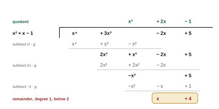
The figure carries out the algorithm for \(f = x^4 + 3x^3 - 2x + 5\) and \(g = x^2 + x - 1\). The first quotient term \(x^2\) cancels \(x^4\), leaving \(2x^3 + x^2 - 2x + 5\); then \(2x\) leaves \(-x^2 + 5\); then \(-1\) leaves \(x + 4\), of degree 1. So \(f = (x^2 + 2x - 1)g + (x + 4)\).

Roots and the factor theorem

Theorem (remainder and factor theorems). Let \(F\) be a field, \(f \in F[x]\) and \(c \in F\). The remainder on dividing \(f\) by \(x - c\) is \(f(c)\). In particular \(c\) is a root of \(f\) if and only if \((x - c)\) divides \(f\).

Proof: divide, \(f = q(x)(x - c) + r\) with \(r\) a constant. Evaluating at \(c\), a homomorphism, gives \(f(c) = q(c) \cdot 0 + r = r\).

Corollary. A nonzero polynomial of degree \(n\) over a field (indeed over an integral domain) has at most \(n\) roots.

Proof: induct on \(n\). If \(c\) is a root, \(f = (x - c)q\) with \(\deg q = n - 1\). Any other root \(d \ne c\) satisfies \(0 = (d - c)q(d)\), and since we are in a domain and \(d - c \ne 0\), \(q(d) = 0\). By induction \(q\) has at most \(n - 1\) roots, so \(f\) has at most \(n\).

The domain hypothesis is essential, as lesson 3 showed with four roots of \(x^2 - 1\) in \(\mathbb{Z}_{12}\). A striking application: in \(\mathbb{Z}_p\), every element satisfies \(a^p = a\) by Fermat's little theorem, so \(x^p - x\) has \(p\) roots, all of \(\mathbb{Z}_p\), and therefore \(x^p - x = \prod_{a \in \mathbb{Z}_p}(x - a)\). Dividing by \(x\) gives \(x^{p - 1} - 1 = \prod_{a \ne 0}(x - a)\), and comparing constant terms yields Wilson's theorem, \((p - 1)! \equiv -1 \pmod p\).

Every ideal of F[x] is principal

Theorem. If \(F\) is a field, every ideal \(I\) of \(F[x]\) is principal: \(I = (g)\), where \(g\) is any nonzero element of \(I\) of least degree (or \(g = 0\) if \(I = \{0\}\)).

Proof: let \(f \in I\) and divide, \(f = qg + r\). Then \(r = f - qg \in I\), and \(r\) has smaller degree than \(g\), so by the choice of \(g\), \(r = 0\). Hence \(f \in (g)\).

This is the same argument that shows every subgroup of \(\mathbb{Z}\) is cyclic, with degree in place of absolute value. It gives greatest common divisors: for \(f, g\) not both zero, the ideal \((f, g)\) equals \((d)\) for a unique monic \(d\), the gcd, and \(d = uf + vg\) for some polynomials \(u, v\). The Euclidean algorithm, repeated division with remainder, computes \(d\), just as for integers: \(\gcd(f, g) = \gcd(g, r)\), and the remainders strictly decrease in degree.

Polynomial arithmetic by computer

The code represents a polynomial as a list of coefficients, constant term first, over \(\mathbb{Q}\) using Fraction, or over \(\mathbb{Z}_p\) by reducing modulo \(p\). It implements multiplication, division with remainder and the Euclidean algorithm, reproduces the division in the figure, and finds a gcd over \(\mathbb{Q}\) and over \(\mathbb{Z}_5\).

from fractions import Fraction as Fr

def trim(f):
    while f and f[-1] == 0:
        f = f[:-1]
    return f

def show(f):
    f = trim(f)
    if not f:
        return "0"
    terms = []
    for i in range(len(f) - 1, -1, -1):
        c = f[i]
        if c == 0:
            continue
        mon = "" if i == 0 else ("x" if i == 1 else f"x^{i}")
        coef = "" if (c == 1 and i) else ("-" if (c == -1 and i) else str(c))
        terms.append(coef + mon)
    return " + ".join(terms).replace("+ -", "- ")

def divmod_poly(f, g, inv=lambda c: 1 / Fr(c), red=lambda c: c):
    f, g = trim([red(c) for c in f]), trim([red(c) for c in g])
    q = [0] * max(len(f) - len(g) + 1, 1)
    lead = inv(g[-1])
    while len(f) >= len(g) and f:
        k = len(f) - len(g)
        c = red(f[-1] * lead)
        q[k] = c
        f = trim([red(f[i] - (c * g[i - k] if i >= k else 0)) for i in range(len(f))])
    return trim(q), f

def gcd_poly(f, g, **kw):
    while trim(g):
        f, g = g, divmod_poly(f, g, **kw)[1]
    lead = kw.get("inv", lambda c: 1 / Fr(c))(f[-1])
    red = kw.get("red", lambda c: c)
    return [red(c * lead) for c in f]

f = [5, -2, 0, 3, 1]          # x^4 + 3x^3 - 2x + 5
g = [-1, 1, 1]                # x^2 + x - 1
q, r = divmod_poly(f, g)
print("q =", show(q), "  r =", show(r))

a = [-6, 11, -6, 1]           # (x-1)(x-2)(x-3)
b = [6, -5, -2, 1]            # (x-1)(x+2)(x-3)
print("gcd over Q:", show(gcd_poly(a, b)))

p = 5
mod = dict(inv=lambda c: pow(int(c), -1, p), red=lambda c: int(c) % p)
u = [1, 0, 0, 0, 1]           # x^4 + 1
v = [3, 0, 1]                 # x^2 + 3
print("gcd over Z_5 of x^4 + 1 and x^2 + 3:", show(gcd_poly(u, v, **mod)))
print("over Z_5, x^4 + 1 =", show(divmod_poly(u, v, **mod)[0]), "times (x^2 + 3)")

q = x^2 + 2x - 1   r = x + 4
gcd over Q: x^2 - 4x + 3
gcd over Z_5 of x^4 + 1 and x^2 + 3: x^2 + 3
over Z_5, x^4 + 1 = x^2 + 2 times (x^2 + 3)

Over \(\mathbb{Q}\), the gcd of \((x - 1)(x - 2)(x - 3)\) and \((x - 1)(x + 2)(x - 3)\) is \((x - 1)(x - 3) = x^2 - 4x + 3\). Over \(\mathbb{Z}_5\), \(x^2 + 3\) divides \(x^4 + 1\): indeed \((x^2 + 3)(x^2 + 2) = x^4 + 5x^2 + 6 \equiv x^4 + 1\). Over \(\mathbb{Q}\), \(x^4 + 1\) is irreducible, so factorization depends on the field, the theme of the next lesson.

Interpolation: the Chinese remainder theorem for polynomials

The analogy between \(\mathbb{Z}\) and \(F[x]\) runs deep enough that the Chinese remainder theorem has a polynomial version. If \(c_1, \ldots, c_n\) are distinct elements of a field \(F\), the polynomials \(x - c_i\) are pairwise coprime, and the map \(F[x] \to F^n\), \(f \mapsto (f(c_1), \ldots, f(c_n))\), is a surjective homomorphism with kernel \(((x - c_1)\cdots(x - c_n))\). By the first isomorphism theorem, \(F[x]/((x - c_1)\cdots(x - c_n)) \cong F \times \cdots \times F\).

Concretely, surjectivity says that any values \(b_1, \ldots, b_n\) are taken by some polynomial, and the uniqueness of the remainder says there is exactly one such polynomial of degree less than \(n\). The idempotents of the Chinese remainder theorem become the Lagrange basis polynomials \(\ell_i(x) = \prod_{j \ne i}\frac{x - c_j}{c_i - c_j}\), which satisfy \(\ell_i(c_i) = 1\) and \(\ell_i(c_j) = 0\) for \(j \ne i\), and the interpolating polynomial is \(\sum b_i\ell_i\). For example, the unique polynomial of degree at most 2 over \(\mathbb{Q}\) with values 1, 3, 7 at 0, 1, 2 is \(x^2 + x + 1\).

Interpolation is not only a classroom exercise. Over a finite field \(\mathbb{Z}_p\), it underlies Shamir's secret-sharing scheme of 1979, in which a secret is the constant term of a random polynomial of degree \(k - 1\) and each participant receives one value: any \(k\) values determine the polynomial, while fewer reveal nothing about the constant term. It also underlies the Reed–Solomon error-correcting codes used on compact discs and in QR codes, which encode a message as the values of a polynomial at many points so that a few corrupted values can be detected and repaired.

Historical note

The division algorithm for polynomials is old; Simon Stevin described the Euclidean algorithm for polynomials in 1585. The formal view of a polynomial as a sequence of coefficients, distinct from the function it defines, became essential once algebraists worked over finite fields, where Galois had computed with polynomials modulo a prime in his 1830 paper on what are now called Galois fields.