
MATH-100 · Lesson 6 of 12 · 37 min
The Mean Value Theorem and the shape of graphs
A derivative tells you the slope of a function at a single point. A great deal of calculus depends on going the other way: using information about the derivative everywhere on an interval to draw conclusions about the function itself. If the derivative is positive throughout an interval, is the function really increasing there? If two functions have the same derivative, how different can they be? The bridge between local slopes and global behavior is the Mean Value Theorem, one of the central results of calculus. This lesson states and interprets the theorem, uses it to justify the tests for increasing and decreasing functions and for concavity, and then combines these tests with limits and asymptotes into a systematic method for sketching graphs. Being able to predict the shape of a function from its formula, and to check a computer plot against that prediction, is a basic engineering skill.
Rolle's theorem
Suppose a function \(f\) is continuous on a closed interval \([a, b]\), differentiable on the open interval \((a, b)\), and takes the same value at both ends, \(f(a) = f(b)\). Rolle's theorem says that there is at least one point \(c\) between \(a\) and \(b\) where \(f'(c) = 0\). The idea is visual: a smooth curve that starts and ends at the same height must turn around somewhere, and at the turning point its tangent is horizontal. The conditions matter. The function \(|x|\) on \([-1, 1]\) has equal endpoint values but no horizontal tangent, because it is not differentiable at 0.
The Mean Value Theorem
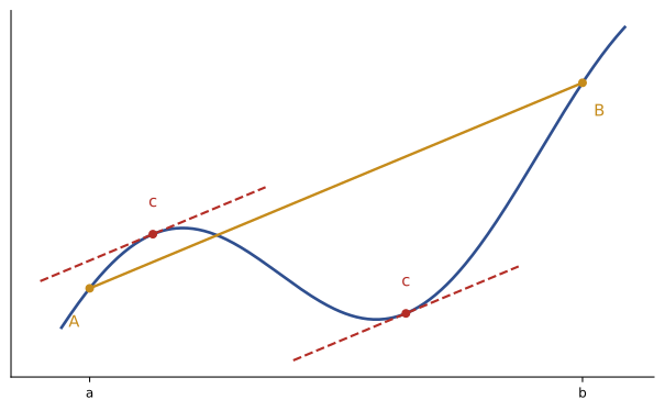
The Mean Value Theorem (MVT) removes the requirement of equal endpoint values. If \(f\) is continuous on \([a, b]\) and differentiable on \((a, b)\), then there is at least one point \(c\) in \((a, b)\) where:
The right side is the slope of the secant line joining the endpoints of the graph, the average rate of change over the interval. The theorem says that somewhere in between, the instantaneous rate equals the average rate: there is a point where the tangent is parallel to the secant. Rolle's theorem is the special case in which the secant is horizontal.
Worked problem
The speed camera argument
Average-speed enforcement systems photograph a vehicle at two points 12 km apart on a highway. A car passes the first at 10:00:00 and the second at 10:06:00. The speed limit is 100 km/h. Can the driver claim never to have exceeded the limit?
Show solution
- Average speed: \(12 \text{ km} / 0.1 \text{ h} = 120\) km/h.
- The car's position is a differentiable function of time, so by the MVT there is an instant when its speed equalled the average, 120 km/h.
Answer: No. At some instant the car was traveling at exactly 120 km/h, even if no single photograph shows it. Section speed control systems in several countries rely on this reasoning.
Worked problem
Finding the point c
For \(f(x) = x^3\) on \([0, 3]\), find all values of \(c\) promised by the MVT.
Show solution
- Average slope: \((27 - 0)/(3 - 0) = 9\).
- Solve \(f'(c) = 3c^2 = 9\): \(c = \sqrt{3} \approx 1.73\), which lies in \((0, 3)\). The negative root is outside the interval.
Answer: c = √3. The theorem guarantees that such a point exists; finding it explicitly is possible only for simple functions, but existence is what the applications need.
Consequences of the Mean Value Theorem
The MVT is rarely used to find numbers. Its importance lies in three consequences that justify much of calculus:
- If \(f'(x) = 0\) for every \(x\) in an interval, then \(f\) is constant on that interval. (Apply the MVT between any two points: the average slope is zero, so the values are equal.)
- If \(f'(x) = g'(x)\) on an interval, then \(f\) and \(g\) differ by a constant: \(f(x) = g(x) + C\). This is why antiderivatives in Lesson 8 always include a "+ C".
- If \(f'(x) > 0\) on an interval, then \(f\) is increasing there; if \(f'(x) < 0\), \(f\) is decreasing.
A further use is bounding errors. If \(|f'(x)| \le M\) on \([a, b]\), the MVT gives \(|f(b) - f(a)| \le M |b - a|\): a function whose slope is bounded cannot change faster than that bound allows.
Worked problem
Bounding an error
A sensor's calibration curve has a slope between 0.95 and 1.05 mV/°C over its whole range. If the temperature reading is wrong by up to 0.4 °C, how far off can the output voltage be?
Show solution
- By the MVT, \(\Delta V = V'(c)\,\Delta T\) for some \(c\), and \(|V'(c)| \le 1.05\).
- So \(|\Delta V| \le 1.05 \times 0.4 = 0.42\) mV.
Answer: At most 0.42 mV. Bounds of this kind, from limits on a derivative, are the basis of error analysis in numerical methods (Lesson 11).
Increasing, decreasing and the first derivative test
Since the sign of \(f'\) determines where \(f\) rises and falls, the intervals of increase and decrease are found by locating the critical points (where \(f' = 0\) or \(f'\) does not exist) and testing the sign of \(f'\) in each interval between them. A sign chart organizes the work.
At a critical point, the change in sign of \(f'\) classifies the point. If \(f'\) changes from positive to negative, \(f\) rises then falls, so the point is a local maximum; from negative to positive, a local minimum; if the sign does not change, neither. This is the first derivative test, which Lesson 7 applies to optimization.
Worked problem
A sign chart
Find where \(f(x) = x^4 - 4x^3\) increases and decreases, and classify its critical points.
Show solution
- \(f'(x) = 4x^3 - 12x^2 = 4x^2(x - 3)\). Critical points: \(x = 0\) and \(x = 3\).
- Signs: for \(x < 0\), \(f' < 0\); for \(0 < x < 3\), \(f' < 0\) (since \(x^2 > 0\) and \(x - 3 < 0\)); for \(x > 3\), \(f' > 0\).
- At \(x = 0\) the sign does not change: neither maximum nor minimum. At \(x = 3\) it changes from negative to positive: a local minimum, \(f(3) = -27\).
Answer: Decreasing on (−∞, 3), increasing on (3, ∞), with a local minimum of −27 at x = 3 and a horizontal tangent but no extremum at x = 0.
Concavity and inflection points
The second derivative describes how the slope itself changes. Where \(f''(x) > 0\), the slope is increasing and the graph is concave up, bending upward like a cup; it lies above its tangent lines. Where \(f''(x) < 0\), the graph is concave down, like a cap, and lies below its tangent lines. A point where the concavity changes is an inflection point.
Concavity has physical meaning. If \(s(t)\) is position, concave up means positive acceleration. For a beam, the curvature of the deflected shape is proportional to the bending moment, so an inflection point in the deflection curve marks where the bending moment is zero. In economics, diminishing returns appear as a concave-down production curve.
At a critical point, the second derivative test classifies the point quickly: if \(f'(c) = 0\) and \(f''(c) > 0\), the graph is a cup and \(c\) is a local minimum; if \(f''(c) < 0\), it is a cap and \(c\) is a local maximum. If \(f''(c) = 0\), the test is inconclusive, as \(x^4\) (a minimum), \(-x^4\) (a maximum) and \(x^3\) (neither) all show at \(x = 0\).
Worked problem
Concavity
Find the intervals of concavity and the inflection points of \(f(x) = x^4 - 4x^3\).
Show solution
- \(f''(x) = 12x^2 - 24x = 12x(x - 2)\), zero at \(x = 0\) and \(x = 2\).
- Signs: positive for \(x < 0\), negative for \(0 < x < 2\), positive for \(x > 2\).
- Concavity changes at both points: inflection points at \((0, 0)\) and \((2, -16)\).
Answer: Concave up on (−∞, 0) and (2, ∞), concave down on (0, 2), with inflection points at (0, 0) and (2, −16). The point x = 0 is both a horizontal tangent and an inflection point.
Asymptotes and end behavior
Limits from Lesson 1 describe the behavior of a graph far from the origin and near points where it blows up:
- Vertical asymptotes occur where \(f(x) \to \pm\infty\) as \(x\) approaches a finite value, typically where a denominator is zero and the numerator is not.
- Horizontal asymptotes are the limits of \(f(x)\) as \(x \to \pm\infty\), when these are finite.
- Slant (oblique) asymptotes occur for rational functions whose numerator degree exceeds the denominator degree by one: polynomial division writes \(f(x) = mx + b + r(x)\) with \(r(x) \to 0\), and the line \(y = mx + b\) is the asymptote.
Exponential and logarithmic terms add their own behavior (Lesson 2): \(e^{-x}\) decays to zero, so functions such as \(x e^{-x}\) approach zero far to the right despite the growing factor \(x\).
A procedure for sketching graphs
Combining these tools gives a reliable procedure:
- Domain: where is the function defined? Note any excluded points.
- Intercepts: find \(f(0)\) and, if practical, the zeros.
- Symmetry: even functions (\(f(-x) = f(x)\)) are symmetric about the \(y\)-axis; odd functions (\(f(-x) = -f(x)\)) are symmetric about the origin.
- Asymptotes: vertical, horizontal and slant.
- First derivative: critical points, intervals of increase and decrease, local extrema.
- Second derivative: concavity and inflection points.
- Plot the key points and join them with a curve consistent with all of the above.
Graphing software can plot any function in an instant, so why learn this? Because software plots only the window you choose and can miss behavior outside it or between sample points, such as a narrow spike near an asymptote or a minimum just outside the window. Knowing what shape to expect lets you choose sensible windows and recognize when a plot is misleading.
Worked problem
A complete sketch
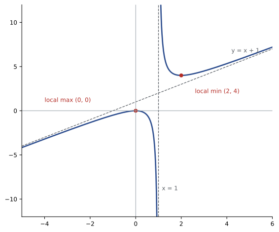
Sketch \(f(x) = \dfrac{x^2}{x - 1}\).
Show solution
- Domain: all \(x \ne 1\). Intercept: \((0, 0)\). No symmetry.
- Vertical asymptote at \(x = 1\): as \(x \to 1^+\), \(f \to +\infty\); as \(x \to 1^-\), \(f \to -\infty\).
- Slant asymptote: division gives \(f(x) = x + 1 + \dfrac{1}{x - 1}\), so \(y = x + 1\).
- First derivative: \(f'(x) = \dfrac{x(x - 2)}{(x - 1)^2}\). Critical points \(x = 0\) and \(x = 2\). \(f' > 0\) for \(x < 0\) and \(x > 2\); \(f' < 0\) on \((0, 1)\) and \((1, 2)\). Local maximum \(f(0) = 0\); local minimum \(f(2) = 4\).
- Second derivative: \(f''(x) = \dfrac{2}{(x - 1)^3}\): concave down for \(x < 1\), concave up for \(x > 1\). No inflection point, because \(x = 1\) is not in the domain.
Answer: Two branches: on the left, a cap rising to a local maximum at (0, 0) and then falling toward −∞ at the asymptote; on the right, a cup descending from +∞ to a local minimum at (2, 4) and then rising along the slant asymptote y = x + 1.
Worked problem
An exponential response
The current in a circuit after a switch closes is \(i(t) = 5t e^{-2t}\) A for \(t \ge 0\). When is it largest, and when is it changing from increasing to decreasing most rapidly (the inflection point)?
Show solution
- \(i'(t) = 5e^{-2t}(1 - 2t)\), zero at \(t = 0.5\) s; \(i' > 0\) before and \(< 0\) after, so a maximum \(i(0.5) = 2.5 e^{-1} = 0.92\) A.
- \(i''(t) = 5e^{-2t}(4t - 4) = 20e^{-2t}(t - 1)\), zero at \(t = 1\) s, where concavity changes from down to up.
- As \(t \to \infty\), \(i \to 0\), since the exponential decay dominates the linear factor.
Answer: A peak of 0.92 A at 0.5 s, an inflection at 1 s (after which the decay slows), and a return toward zero. This shape is typical of critically damped circuits and of drug concentration after a dose.
Common mistakes
MistakeApplying the MVT to a function that is not differentiable on the interval.
InsteadCheck continuity on [a, b] and differentiability on (a, b) first.
MistakeConcluding that f′(c) = 0 means a maximum or minimum.
InsteadCheck whether f′ changes sign; x³ has f′(0) = 0 and no extremum.
MistakeDeclaring an inflection point wherever f″ = 0.
InsteadConcavity must actually change; x⁴ has f″(0) = 0 but no inflection.
MistakePlacing an inflection point at a vertical asymptote.
InsteadPoints outside the domain cannot be inflection points.
MistakeTrusting a single computer plot window.
InsteadUse asymptotes and critical points to choose windows and check the plot.
Summary and key terms
- Rolle's theorem: equal endpoint values imply a horizontal tangent somewhere between.
- The Mean Value Theorem: somewhere, the instantaneous rate equals the average rate.
- Consequences: zero derivative means constant; equal derivatives differ by a constant; sign of f′ gives increase or decrease.
- Bounds on f′ bound changes in f, which underlies error analysis.
- The first derivative test classifies critical points by the sign change of f′.
- f″ > 0 means concave up and f″ < 0 concave down; inflection points are where concavity changes.
- Domain, intercepts, symmetry, asymptotes, f′ and f″ combine into a reliable sketch.
- Rolle's theorem
- Equal endpoint values guarantee a point with zero derivative between them.
- Mean Value Theorem
- A differentiable function has a point where its slope equals its average rate of change.
- Secant line
- A line through two points on a graph.
- Critical point
- A point where f′ is zero or undefined.
- First derivative test
- Classifying critical points by sign changes of f′.
- Concave up
- Curving upward, with f″ > 0.
- Inflection point
- A point where concavity changes.
- Second derivative test
- Classifying a critical point by the sign of f″.
- Slant asymptote
- A non-horizontal line that a graph approaches far from the origin.
- Sign chart
- A table of the signs of a derivative on intervals between critical points.
Practice problems
Work each problem on paper first, then reveal the answer to check.
Verify Rolle's theorem for \(f(x) = x^2 - 4x\) on \([0, 4]\).
Show answer
f(0) = f(4) = 0; f′(c) = 2c − 4 = 0 at c = 2.
Find c from the MVT for \(f(x) = \sqrt{x}\) on \([0, 4]\).
Show answer
Average slope 1/2; 1/(2√c) = 1/2 gives c = 1.
A car travels 150 km in 1.5 h. What does the MVT guarantee?
Show answer
At some instant its speed was exactly 100 km/h.
If \(f'(x) = 2x\) and \(f(0) = 3\), what is f?
Show answer
f(x) = x² + 3.
Where is \(f(x) = x^3 - 12x\) increasing?
Show answer
x < −2 and x > 2.
Classify the critical points of \(x^3 - 12x\).
Show answer
Local maximum 16 at x = −2; local minimum −16 at x = 2.
Find the inflection point of \(x^3 - 6x^2 + 5\).
Show answer
f″ = 6x − 12, so x = 2; point (2, −11).
Find all asymptotes of \(\dfrac{2x + 1}{x - 3}\).
Show answer
Vertical x = 3; horizontal y = 2.
Find the slant asymptote of \(\dfrac{x^2 + 1}{x}\).
Show answer
y = x.
Where is \(t e^{-t}\) largest for \(t \ge 0\)?
Show answer
At t = 1, value 1/e.
Lesson quiz · 5 questions
Score 60% or more to complete this lesson.
Create a free account to save your progress, take quizzes and earn a certificate.