
MATH-100 · Lesson 11 of 12 · 32 min
Taylor polynomials, approximation and numerical error
Engineers approximate all the time. A pendulum's period is calculated with \(\sin\theta \approx \theta\); the sag of a power line is modeled as a parabola instead of a catenary; a nonlinear sensor is linearized around its operating point; a computer evaluates \(e^x\) by adding a few terms of a polynomial. Every approximation carries an error, and good engineering requires knowing how big that error is. Earlier lessons used the tangent line as an approximation (Lesson 3), finite differences to estimate derivatives from data (Lesson 3), Newton's method to solve equations (Lesson 7), and the trapezoid rule to integrate data (Lesson 9). This lesson develops the idea behind all of them: Taylor polynomials, which approximate a function near a point by matching its derivatives, together with a formula for the error. It then uses that formula to explain how accurate numerical methods are, and closes with the limits imposed by the finite precision of computer arithmetic.
From tangent lines to Taylor polynomials
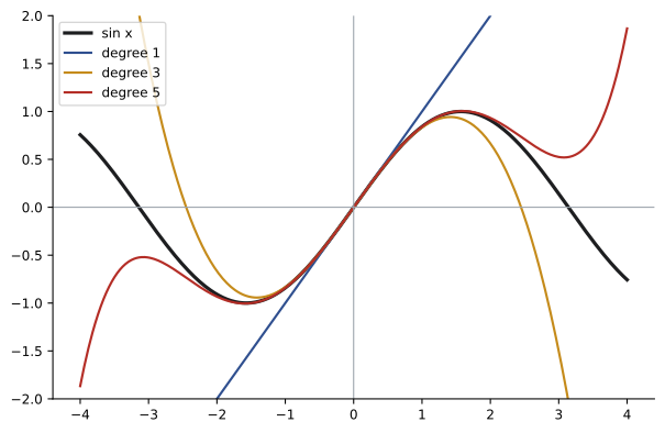
The linear approximation \(f(x) \approx f(a) + f'(a)(x - a)\) matches the function's value and slope at \(a\). It works well very close to \(a\) but drifts away as the curve bends. A better approximation should also match the bending, that is, the second derivative. The quadratic polynomial that matches \(f\), \(f'\) and \(f''\) at \(a\) is:
Continuing the pattern, the Taylor polynomial of degree \(n\) matches the first \(n\) derivatives:
where \(f^{(k)}\) is the \(k\)-th derivative and \(k! = 1 \cdot 2 \cdots k\) is \(k\) factorial (with \(0! = 1\)). The factorials appear because the \(k\)-th derivative of \((x - a)^k\) is \(k!\). When \(a = 0\), the polynomial is often called a Maclaurin polynomial.
Worked problem
Taylor polynomials of eˣ
Find the Taylor polynomials of degree 1, 2 and 4 for \(e^x\) at \(a = 0\), and use them to estimate \(e^{0.5}\) (exact value 1.648 72).
Show solution
- Every derivative of \(e^x\) is \(e^x\), which equals 1 at 0. So \(P_n(x) = 1 + x + \dfrac{x^2}{2!} + \cdots + \dfrac{x^n}{n!}\).
- \(P_1(0.5) = 1.5\); \(P_2(0.5) = 1.625\); \(P_4(0.5) = 1 + 0.5 + 0.125 + 0.020\,83 + 0.002\,60 = 1.648\,44\).
Answer: Errors of 0.149, 0.024 and 0.000 28: each extra term improves the estimate substantially. Calculators and computer libraries evaluate exponentials with polynomial approximations of this kind, combined with tricks that keep x small.
The most frequently used Taylor polynomials, all centered at 0, are:
The last, the binomial approximation, is particularly useful: \(\sqrt{1 + x} \approx 1 + x/2\) and \(1/(1 + x) \approx 1 - x\) for small \(x\).
Engineering approximations
Many standard engineering formulas are Taylor approximations in disguise:
- The small-angle approximation \(\sin\theta \approx \theta\) (with \(\theta\) in radians) gives the simple pendulum period \(T = 2\pi\sqrt{L/g}\) and the linear theory of beam deflection. It is accurate to within 1 percent up to about 14° (0.24 rad), since the next term, \(\theta^3/6\), is then about 1 percent of \(\theta\).
- A cable hanging under its own weight forms a catenary, \(y = a\cosh(x/a)\). Expanding \(\cosh u \approx 1 + u^2/2\) gives a parabola, \(y \approx a + x^2/(2a)\), which is why power line sag calculations use parabolas when the sag is small compared with the span.
- The relativistic and quantum corrections that engineers occasionally meet are usually the second term of a Taylor expansion, which is why they are negligible at ordinary speeds and energies.
- Linearizing a nonlinear device around its operating point, as in transistor amplifiers, valve flow characteristics or the small-signal converter models of ELE-470, uses the first-order Taylor polynomial in each variable.
Worked problem
Accuracy of the small-angle approximation
A pendulum swings to an amplitude of 20°. Estimate the error made by replacing \(\sin\theta\) with \(\theta\) at the extreme of the swing.
Show solution
- \(\theta = 20° = 0.349\) rad. \(\sin 0.349 = 0.342\).
- Relative error: \((0.349 - 0.342)/0.342 = 2.0\) percent, close to the estimate \(\theta^2/6 = 0.0203\).
Answer: About 2 percent at the extreme of the swing, less elsewhere. The actual period of a 20° pendulum is about 0.8 percent longer than the small-angle formula predicts, an error that mattered to clockmakers.
Worked problem
Sag of a power line
A conductor spans 300 m between supports at equal height and hangs as a catenary with \(a = 1{,}500\) m. Compare the exact sag \(a(\cosh(150/a) - 1)\) with the parabolic approximation \(150^2/(2a)\).
Show solution
- Parabolic: \(22{,}500 / 3{,}000 = 7.500\) m.
- Exact: \(u = 0.1\); \(\cosh 0.1 = 1.005\,004\); sag \(= 1500 \times 0.005\,004 = 7.506\) m.
Answer: The parabola gives 7.500 m against an exact 7.506 m, an error of less than 0.1 percent, because the neglected term, u⁴/24, is tiny when the sag is small compared with the span.
How big is the error?
Taylor's theorem gives the error of the approximation. If \(f\) has \(n + 1\) derivatives, then for each \(x\) there is a point \(c\) between \(a\) and \(x\) such that:
This is the Lagrange form of the remainder, a generalization of the Mean Value Theorem of Lesson 6 (which is the case \(n = 0\)). We do not know \(c\), but if \(|f^{(n+1)}| \le M\) between \(a\) and \(x\), then the error is at most \(M|x - a|^{n+1}/(n + 1)!\). Two lessons follow. The error shrinks rapidly as \(x\) approaches \(a\), like the \((n + 1)\)-th power of the distance. And the factorial in the denominator makes high-degree polynomials very accurate for well-behaved functions.
Worked problem
Choosing the degree
How many terms of the Taylor polynomial of \(\sin x\) at 0 are needed to compute \(\sin(0.5)\) with an error below \(10^{-6}\)?
Show solution
- All derivatives of \(\sin x\) are bounded by 1, so the error of \(P_n\) is at most \(0.5^{n+1}/(n + 1)!\).
- \(n = 5\): \(0.5^6/720 = 2.2 \times 10^{-5}\), too large. \(n = 7\): \(0.5^8/40{,}320 = 9.7 \times 10^{-8}\), small enough.
- Since \(\sin x\) has only odd powers, \(P_7 = x - x^3/6 + x^5/120 - x^7/5040\) has four non-zero terms.
Answer: Four terms give sin(0.5) to better than 10⁻⁶. Error bounds of this kind are how numerical libraries guarantee their accuracy. MATH-101 extends Taylor polynomials to infinite Taylor series.
Why numerical methods work, and how well
Taylor's theorem explains the accuracy of the numerical methods met in earlier lessons.
Finite differences
Expanding \(f(x + h) = f(x) + hf'(x) + \tfrac{h^2}{2}f''(x) + \tfrac{h^3}{6}f'''(x) + \cdots\) and rearranging shows that the forward difference has an error of about \(\tfrac{h}{2}f''(x)\), proportional to \(h\). Writing the same expansion for \(f(x - h)\) and subtracting cancels the \(h^2\) terms, so the central difference has an error of about \(\tfrac{h^2}{6}f'''(x)\), proportional to \(h^2\). This is why the central difference in Lesson 3 was about fifty times more accurate with the same step: halving \(h\) halves the forward error but quarters the central error. A method whose error is proportional to \(h^p\) is said to be of order \(p\).
Numerical integration
The trapezoid rule is of order 2: its error over a fixed interval is approximately \(-\tfrac{(b - a)h^2}{12}f''\), so halving the step reduces the error by a factor of four. Simpson's rule, which fits parabolas through groups of three points, is of order 4, so halving the step reduces its error by a factor of sixteen. Knowing the order allows a powerful trick, Richardson extrapolation: if \(T_h\) and \(T_{h/2}\) are trapezoid estimates with step \(h\) and \(h/2\), the combination \((4T_{h/2} - T_h)/3\) cancels the leading error term.
Worked problem
Richardson extrapolation
The trapezoid rule for \(\int_0^1 e^x\,dx\) (exact value \(e - 1 = 1.718\,282\)) gives 1.753 931 with 2 intervals and 1.727 222 with 4 intervals. Improve the estimate.
Show solution
- Errors: 0.0356 and 0.0089, a ratio of 4, as expected for order 2.
- Extrapolate: \((4 \times 1.727\,222 - 1.753\,931)/3 = 1.718\,319\).
Answer: The extrapolated value 1.718 319 has an error of only 0.000 037, better than the trapezoid rule would achieve with about 60 intervals. This combination is exactly Simpson's rule, and repeating the idea gives Romberg integration.
Newton's method
Lesson 7 observed that Newton's method roughly doubles the number of correct digits at each step. Taylor's theorem explains why: expanding \(f\) around the current estimate shows that the new error is proportional to the square of the old error, \(e_{n+1} \approx \tfrac{f''(r)}{2f'(r)}e_n^2\). This quadratic convergence holds once the estimate is close to a simple root. Far from the root, or where \(f'\) is small, the method can overshoot, cycle or diverge, which is why practical solvers combine Newton steps with safeguards such as bisection.
Round-off error and floating-point arithmetic
Computers store numbers in floating-point form with a fixed number of significant digits. Standard double-precision arithmetic carries about 16 significant decimal digits; the gap between 1 and the next representable number, called machine epsilon, is about \(2.2 \times 10^{-16}\). Every arithmetic operation rounds its result, introducing a relative error of up to about \(10^{-16}\). Usually this is negligible, but two situations magnify it.
Catastrophic cancellation
Subtracting two nearly equal numbers loses the digits they share. For \(x = 10^{-8}\), \(\cos x = 0.999\,999\,999\,999\,999\,95\), which rounds to exactly 1 in double precision, so computing \(1 - \cos x\) gives 0 instead of the correct \(5 \times 10^{-17}\). Rewriting the expression avoids the subtraction: \(1 - \cos x = 2\sin^2(x/2)\), which computes accurately. The Taylor polynomial \(x^2/2\) gives the answer too. The same problem appears in the quadratic formula when \(b^2 \gg 4ac\), in computing small differences of large measured quantities, and in variance calculations.
Truncation versus round-off
In a finite difference, the truncation error (from the approximation) shrinks as \(h\) gets smaller, but the round-off error grows, because the numerator \(f(x + h) - f(x)\) is a difference of nearly equal numbers, each carrying a rounding error of about \(\varepsilon |f|\), divided by a small \(h\). The total error is roughly \(\tfrac{h}{2}|f''| + \tfrac{2\varepsilon |f|}{h}\), smallest when \(h\) is about \(\sqrt{\varepsilon}\), around \(10^{-8}\) for a forward difference in double precision. Making \(h\) smaller than this makes the answer worse, not better. Measured data, whose noise is far larger than machine epsilon, has a much larger optimal step, which is why noisy data must be smoothed before differentiation.
| Step h | Forward-difference estimate of d/dx eˣ at x = 1 | Error |
|---|---|---|
| 10⁻² | 2.731 919 | 1.4 × 10⁻² |
| 10⁻⁴ | 2.718 418 | 1.4 × 10⁻⁴ |
| 10⁻⁶ | 2.718 283 | 1.4 × 10⁻⁶ |
| 10⁻⁸ | 2.718 282 | about 10⁻⁸ to 10⁻⁷ |
| 10⁻¹⁰ | 2.718 28… | about 10⁻⁶ (round-off) |
| 10⁻¹² | 2.718 … | about 10⁻⁴ (round-off) |
Approximation as an engineering habit
The tools of this lesson support habits that every engineer needs. Before trusting a computed result, estimate it roughly by hand using linear or quadratic approximations. When using a numerical method, check convergence by repeating the calculation with a smaller step or tighter tolerance and confirming that the answer settles down at the expected rate. When a formula involves subtracting nearly equal quantities, look for a rearrangement. And when an approximation such as the small-angle formula is used, check the size of the first neglected term: if it is small compared with the required accuracy, the approximation is safe.
Common mistakes
MistakeUsing the small-angle approximation with angles in degrees.
Insteadsin θ ≈ θ holds only with θ in radians.
MistakeForgetting the factorials in Taylor coefficients.
InsteadThe k-th term is f⁽ᵏ⁾(a)(x − a)ᵏ/k!.
MistakeAssuming a Taylor polynomial is accurate far from its center.
InsteadUse the remainder to check the error at the distance required.
MistakeMaking the finite-difference step as small as possible.
InsteadBelow about √ε round-off dominates; with noisy data the optimal step is larger still.
MistakeSubtracting nearly equal numbers without thinking.
InsteadRearrange formulas to avoid catastrophic cancellation.
Summary and key terms
- Taylor polynomials match a function's value and first n derivatives at a point.
- Key expansions: eˣ, sin x, cos x, ln(1 + x) and the binomial (1 + x)ᵖ.
- Small-angle, parabolic-sag and linearized models are Taylor approximations.
- The Lagrange remainder bounds the error by M|x − a|ⁿ⁺¹/(n + 1)!.
- Forward differences are order 1, central differences and the trapezoid rule order 2, Simpson's rule order 4.
- Richardson extrapolation cancels the leading error; Newton's method converges quadratically near a root.
- Double precision carries about 16 digits; cancellation and tiny steps amplify round-off error.
- Taylor polynomial
- A polynomial matching a function's derivatives at a point.
- Maclaurin polynomial
- A Taylor polynomial centered at 0.
- Factorial
- The product k! = 1·2·…·k.
- Lagrange remainder
- A formula for the error of a Taylor polynomial.
- Order of a method
- The power p in an error proportional to hᵖ.
- Truncation error
- Error from approximating a mathematical process.
- Richardson extrapolation
- Combining estimates at two step sizes to cancel the leading error.
- Quadratic convergence
- Error at each step proportional to the square of the previous error.
- Machine epsilon
- The relative spacing of floating-point numbers near 1.
- Catastrophic cancellation
- Loss of significant digits when subtracting nearly equal numbers.
Practice problems
Work each problem on paper first, then reveal the answer to check.
Find the degree-2 Taylor polynomial of \(\cos x\) at 0 and estimate \(\cos 0.2\).
Show answer
1 − x²/2; 0.98 (exact 0.980 07).
Use the binomial approximation to estimate \(\sqrt{1.04}\).
Show answer
1 + 0.02 = 1.02 (exact 1.019 80).
Estimate \(\ln(1.1)\) with two terms.
Show answer
0.1 − 0.005 = 0.095 (exact 0.095 31).
Find the degree-2 Taylor polynomial of \(\sqrt{x}\) at \(a = 4\).
Show answer
2 + (x − 4)/4 − (x − 4)²/64.
Up to what angle is sin θ ≈ θ accurate to 0.5%?
Show answer
θ²/6 = 0.005, θ ≈ 0.17 rad ≈ 10°.
Bound the error of \(e^x \approx 1 + x + x^2/2\) at \(x = 0.1\).
Show answer
At most e^0.1 × 0.001/6 ≈ 1.8 × 10⁻⁴.
A method of order 2 has error 0.008 with step h. Error with step h/2?
Show answer
About 0.002.
Trapezoid estimates are 2.10 (h) and 2.04 (h/2). Richardson estimate?
Show answer
(4 × 2.04 − 2.10)/3 = 2.02.
Newton error is 10⁻³ at one step. Roughly what next (with factor about 1)?
Show answer
About 10⁻⁶.
Rewrite \(\sqrt{x + 1} - \sqrt{x}\) to avoid cancellation for large x.
Show answer
1/(√(x + 1) + √x).
Lesson quiz · 5 questions
Score 60% or more to complete this lesson.
Create a free account to save your progress, take quizzes and earn a certificate.