
GEOM-300 · Lesson 5 of 12 · 23 min
Error sources
On the third day of the canal survey, a geomagnetic storm reached the prairies. The aurora was visible from the field office in the evening, and during the afternoon the RTK rovers kept losing their fixed solutions. Theo Martel's static sessions from that day showed residuals two or three times larger than usual. Ruth Albrecht used the day to make a point to the crew: every GNSS error has a physical cause, a typical size and a remedy, and good practice consists of knowing which errors matter for the job at hand and how each is reduced or eliminated. This lesson goes through them one by one, from the satellites to the receiver, and ends with an error budget.
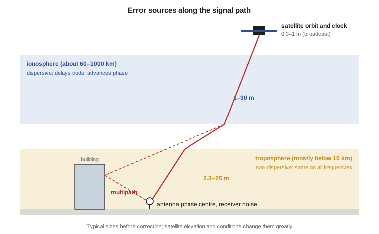
Satellite orbit and clock errors
The broadcast orbit and clock are predictions, and their combined effect along the line of sight, the signal-in-space range error, is typically 0.3 to 1 m for GPS and Galileo today. The clock part dominates, because an atomic clock that is predicted well for an hour can drift by nanoseconds over several hours. The orbit error is mostly along-track and cross-track, and only part of it projects onto the line of sight. Both errors are common to all users who see the satellite, so they cancel almost completely in relative positioning over short baselines, and they are replaced by precise products for precise point positioning. Occasionally a satellite clock jumps or a satellite is maneuvered without being flagged in time; such faults are rare but can produce errors of tens or hundreds of meters, and they are the reason integrity monitoring exists.
The ionosphere
The ionosphere is the region of the upper atmosphere, roughly 60 to 1000 km up, where solar ultraviolet and X-ray radiation ionizes the thin gas and free electrons persist. The electrons slow the code and advance the carrier phase by \(40.3\,\text{TEC}/f^2\) meters, where TEC is the total electron content along the path, measured in TEC units of \(10^{16}\) electrons per square meter. One TEC unit delays the L1 code by 0.162 m. Vertical TEC over mid-latitudes ranges from a few units at night to 20 to 60 units in the early afternoon, depending on season and on the eleven-year solar cycle, whose recent maximum fell around 2024 and 2025. Under storm conditions TEC can rise much higher and vary sharply over short distances.
A slanted path through the ionosphere is longer than a vertical one. With the common thin-shell model, which concentrates all electrons in a layer at about 350 km, the slant TEC is the vertical TEC divided by the cosine of the zenith angle at the point where the signal pierces the shell, which gives an obliquity factor of up to about three at low elevations.
Single-frequency receivers correct the ionosphere with a broadcast model. GPS broadcasts the eight coefficients of the Klobuchar model, which describes the vertical delay as a half-cosine in local time; it typically removes about half of the delay. Galileo broadcasts coefficients for the NeQuick model, which is somewhat better. Dual-frequency receivers do far better by measuring the delay directly and forming the ionosphere-free combination, which removes the first-order effect completely. Second-order effects, caused by the Earth's magnetic field, amount to a few millimeters to a centimeter or two and are modeled only in the most precise processing.
At high latitudes, and therefore occasionally over Alberta and Montana when the auroral oval expands during storms, irregularities in the ionosphere cause scintillation: rapid fluctuations of amplitude and phase. Phase scintillation can make receivers lose lock and slip cycles on many satellites at once, which is what broke the RTK fixes on the storm day. Space weather services of Natural Resources Canada and of the United States National Oceanic and Atmospheric Administration publish forecasts and alerts; for critical work it is worth checking them before going to the field.
Worked problem
Slant ionospheric delay
The vertical TEC above CR1 in the early afternoon is 20 TEC units. A satellite is at 30° elevation. Using a thin shell at 350 km and an Earth radius of 6371 km, find the slant delay on L1 (1575.42 MHz) and on L5 (1176.45 MHz).
Show solution
- \[\sin z' = \frac{R}{R + h}\cos E = \frac{6371}{6721} \times \cos 30^\circ = 0.820\,93, \qquad z' = 55.18^\circ\]
- \[\text{STEC} = \frac{\text{VTEC}}{\cos z'} = \frac{20}{0.571\,0} = 35.03\ \text{TECU}\]
- \[I_1 = \frac{40.3 \times 35.03 \times 10^{16}}{(1.575\,42 \times 10^{9})^2} = 5.69\ \text{m}\]
- \[I_5 = I_1 \big(\tfrac{f_1}{f_5}\big)^2 \text{ with } \tfrac{f_1}{f_5} = 1.3391: \quad I_5 = 5.69 \times 1.7933 = 10.20\ \text{m}\]
Answer: The L1 code is delayed by about 5.7 m and the L5 code by about 10.2 m. The carrier phases are advanced by the same amounts. A broadcast model removing half the delay would leave almost 3 m on L1, which is why single-frequency stand-alone positions are limited to a few meters.
The troposphere
Below about 50 km, and mostly in the lowest 10 km, the neutral atmosphere delays all GNSS signals equally on every frequency, so the delay cannot be removed by combining frequencies. The zenith delay has two parts. The hydrostatic or dry part, about 2.3 m at sea level, depends on surface pressure and can be computed to a millimeter or two from it, for example with the Saastamoinen formula. It is smaller at higher sites because there is less atmosphere above them. The wet part, caused by water vapor, is typically 5 to 30 cm, varies quickly in space and time, and cannot be predicted accurately from surface measurements. Over the dry prairies it is often under 10 cm; in a humid summer thunderstorm it can exceed 25 cm.
The slant delay is the zenith delay multiplied by a mapping function of elevation, roughly \(1/\sin E\) at high elevations but growing more slowly than that near the horizon because of the Earth's curvature. Precise work uses separate hydrostatic and wet mapping functions derived from numerical weather models, such as the Vienna mapping functions or their empirical approximations. In precise processing the residual zenith wet delay is estimated as an unknown parameter every hour or so, together with horizontal gradients; the estimates are so good that they are used in weather forecasting.
The program below computes the standard-atmosphere pressure at CR1, about 898 hPa at 1005 m, the Saastamoinen hydrostatic and wet zenith delays, and the slant delay at several elevations with a simple mapping function. It then computes the L1 ionospheric delay for three levels of vertical TEC and three elevations, and finally combines typical range error sizes into a user equivalent range error.
# Atmospheric delays at the site and a user range error budget
import math

LAT, H = 47.5060042, 1004.826                    # pillar CR1, ellipsoidal height used for the model
# Standard atmosphere at the site height
P = 1013.25 * (1 - 2.2557e-5 * H) ** 5.2568       # pressure, hPa
T = 288.15 - 0.0065 * H                          # temperature, K
e = 8.0                                          # partial pressure of water in the air on a dry prairie day, hPa
phi = math.radians(LAT)
zhd = 0.0022768 * P / (1 - 0.00266 * math.cos(2 * phi) - 0.00028 * H / 1000)   # Saastamoinen hydrostatic
zwd = 0.002277 * (1255 / T + 0.05) * e                                          # Saastamoinen wet
print("pressure", round(P, 1), "hPa  zenith hydrostatic", round(zhd, 3), "m  zenith wet", round(zwd, 3), "m")

def mapping(el_deg):                              # a simple continued-fraction style mapping function
    s = math.sin(math.radians(el_deg))
    return 1.0 / (s + 0.00143 / (math.tan(math.radians(el_deg)) + 0.0445))

for el in (90, 45, 30, 15, 10, 5):
    print("elevation", str(el).rjust(2), "deg  mapping", format(mapping(el), "6.3f"),
          "  slant troposphere", format((zhd + zwd) * mapping(el), "6.3f"), "m")

# Ionosphere: vertical TEC with a thin-shell obliquity factor at 350 km
R_E, h_ion = 6371.0, 350.0
f1 = 1575.42e6
for vtec in (5, 20, 60):
    for el in (90, 30, 10):
        z = math.asin(R_E / (R_E + h_ion) * math.cos(math.radians(el)))
        stec = vtec * 1e16 / math.cos(z)
        print("VTEC", str(vtec).rjust(2), "TECU, el", str(el).rjust(2), "deg: L1 delay", format(40.3 * stec / f1 ** 2, "6.2f"), "m")

# User equivalent range error (1 sigma, m) for a single-frequency and a dual-frequency receiver
budget = {
    "single-frequency": {"satellite clock and orbit": 0.6, "ionosphere after broadcast model": 2.5,
                         "troposphere after model": 0.2, "multipath": 0.6, "receiver noise": 0.3},
    "dual-frequency": {"satellite clock and orbit": 0.6, "ionosphere residual (ionosphere-free)": 0.1,
                       "troposphere after model": 0.2, "multipath": 0.6, "receiver noise": 0.5},
}
for mode, items in budget.items():
    uere = math.sqrt(sum(v * v for v in items.values()))
    print(mode, "UERE", round(uere, 2), "m -> horizontal 95 % with HDOP 0.94:", round(2 * 0.94 * uere, 1), "m;",
"vertical 95 % with VDOP 1.47:", round(2 * 1.47 * uere, 1), "m")pressure 898.2 hPa zenith hydrostatic 2.045 m zenith wet 0.082 m elevation 90 deg mapping 1.000 slant troposphere 2.127 m elevation 45 deg mapping 1.411 slant troposphere 3.003 m elevation 30 deg mapping 1.991 slant troposphere 4.235 m elevation 15 deg mapping 3.797 slant troposphere 8.076 m elevation 10 deg mapping 5.552 slant troposphere 11.810 m elevation 5 deg mapping 10.205 slant troposphere 21.709 m VTEC 5 TECU, el 90 deg: L1 delay 0.81 m VTEC 5 TECU, el 30 deg: L1 delay 1.42 m VTEC 5 TECU, el 10 deg: L1 delay 2.26 m VTEC 20 TECU, el 90 deg: L1 delay 3.25 m VTEC 20 TECU, el 30 deg: L1 delay 5.69 m VTEC 20 TECU, el 10 deg: L1 delay 9.06 m VTEC 60 TECU, el 90 deg: L1 delay 9.74 m VTEC 60 TECU, el 30 deg: L1 delay 17.06 m VTEC 60 TECU, el 10 deg: L1 delay 27.17 m single-frequency UERE 2.66 m -> horizontal 95 % with HDOP 0.94: 5.0 m; vertical 95 % with VDOP 1.47: 7.8 m dual-frequency UERE 1.01 m -> horizontal 95 % with HDOP 0.94: 1.9 m; vertical 95 % with VDOP 1.47: 3.0 m
The zenith tropospheric delay at CR1 is about 2.13 m, of which only 8 cm is wet on a dry day. At 15° elevation the slant delay is already 8.1 m, and at 5° it is 22 m, which shows why low satellites need good mapping functions or should be excluded. The ionosphere spans a much wider range, from under a meter at night overhead to 27 m at low elevation under very high TEC. Combined into a budget, a single-frequency receiver has a UERE of about 2.7 m, giving 95 % horizontal accuracy of about 5 m with the HDOP of Lesson 4, while a dual-frequency receiver has about 1 m and 2 m.
Multipath
Multipath is the arrival of reflected copies of a signal along with the direct one. The reflected signal travels a longer path and distorts the correlation peak, biasing the code measurement. Code multipath can reach several meters near large reflectors such as metal buildings, vehicles, fences and water surfaces, though it is usually a few decimeters in good sites. Carrier phase multipath is much smaller, limited to a quarter of a wavelength, about 5 cm, and usually a few millimeters, but it does not average out quickly: for a static antenna the reflection geometry changes slowly with the satellite's motion, so multipath appears as errors with periods of minutes, and with GPS it repeats every sidereal day.
Mitigation starts with site selection: avoid reflecting surfaces near the antenna, especially above it, and avoid setting up next to vehicles. Antenna design helps: geodetic antennas with ground planes or choke rings attenuate signals arriving from below the horizon and left-hand circularly polarized reflections. Receiver correlator designs reduce code multipath, and modern wideband signals such as L5 and Galileo E5 are inherently more resistant. Long observation sessions average the remaining errors, and elevation masks remove the satellites most affected. For permanent stations, multipath maps can be estimated and removed.
Receiver, antenna and hardware effects
Receiver noise in the tracking loops is typically a few decimeters for C/A code, a few centimeters for modern codes, and about a millimeter for carrier phase. Hardware delays in satellites and receivers differ between signals; for code they are expressed as differential code biases, a few nanoseconds, which affect single-frequency users and ionosphere estimation and are published by analysis centers. For carrier phase, the corresponding biases are what stop simple ambiguity resolution in precise point positioning and are the subject of Lesson 9. Antenna phase center offsets and variations, introduced in Lesson 2, must be applied with calibrations, especially when different antenna types are combined. Finally, because GNSS signals are right-hand circularly polarized, rotating either antenna changes the measured phase; this phase wind-up is a few centimeters per rotation and matters for precise point positioning, where satellite antennas rotate as the satellites turn to keep their solar panels facing the Sun.
The moving ground
A geodetic receiver bolted to a pillar is not stationary. The solid Earth tide raises and lowers the ground by up to about 30 cm twice a day, with horizontal motions of a few centimeters. Ocean tides load the crust and depress coastal sites by up to several centimeters; inland in Alberta and Montana this ocean loading is only a few millimeters. The changing rotation axis causes a pole tide of up to about a centimeter. These effects are computed from conventional models and applied to coordinates so that a station's position refers to a conventional tide-free or mean-tide crust. Over a short baseline they are almost identical at both ends and cancel; for precise point positioning they must be modeled. Long-term plate motion, about 2 to 3 cm per year relative to the ITRF in North America, and slow vertical motions such as glacial isostatic adjustment are handled by reference frames and epochs, discussed in Lesson 9.
The error budget
| Error source | Size before correction | Single-frequency, after models | Dual-frequency or differential |
|---|---|---|---|
| Satellite orbit and clock (broadcast) | 0.3–1 m | 0.3–1 m | cancels over short baselines; 2–5 cm with precise products |
| Ionosphere | 1–30 m at L1 | 1–5 m (broadcast model) | first order removed; mm to cm residual |
| Troposphere | 2.3–25 m | 0.1–0.5 m (model) | cancels over short baselines; mm with estimation |
| Code multipath | 0.1–5 m | same | reduced by smoothing and antenna design |
| Phase multipath | 1–50 mm | same | averages with time; does not cancel |
| Receiver noise (code / phase) | 0.05–0.5 m / 1 mm | same | same |
| Antenna phase center | mm to cm | mm to cm | removed with calibrations |
| Solid Earth tide | up to 0.3 m | usually ignored | cancels over short baselines; modeled in PPP |
The budget explains the hierarchy of methods in the rest of this course. Stand-alone single-frequency positioning is limited by the ionosphere to a few meters; dual-frequency stand-alone positioning by broadcast orbits, clocks and code multipath to a meter or two. Differential code methods remove most of the common errors and reach decimeters to a meter. Carrier-phase methods, relative or with precise products, reach centimeters and millimeters, limited in the end by multipath, antenna models, the troposphere and the treatment of ambiguities.
Common mistakes
MistakeRemoving the troposphere with two frequencies.
InsteadThe troposphere is non-dispersive at GNSS frequencies; it must be modeled or estimated.
MistakeAssuming the broadcast ionospheric model removes the ionosphere.
InsteadThe Klobuchar model removes about half the delay; dual-frequency observations remove the first-order effect.
MistakeSetting up beside a vehicle or metal building.
InsteadReflections cause code multipath of meters and phase multipath of millimeters to centimeters; choose open, reflection-free sites.
MistakeExpecting phase multipath to average out in a few minutes.
InsteadIt varies with satellite geometry over tens of minutes; long sessions or repeat days are needed.
MistakeIgnoring space weather.
InsteadGeomagnetic storms raise TEC and cause scintillation, cycle slips and lost RTK fixes; check forecasts for critical work.
Summary and key terms
- Broadcast orbit and clock errors are typically 0.3–1 m and cancel over short baselines.
- The ionosphere delays code and advances phase by 40.3 TEC/f²; dual-frequency combinations remove it.
- Broadcast models such as Klobuchar remove about half the ionospheric delay.
- The tropospheric delay is about 2.3 m at the zenith at sea level, mostly hydrostatic; the wet part is hard to predict and is estimated.
- Mapping functions scale zenith delays to slant delays; low-elevation delays exceed 10 m.
- Multipath biases code by up to meters and phase by millimeters; site selection and antenna design mitigate it.
- Earth tides, loading and plate motion move the ground and must be modeled for precise work.
- TEC
- Total electron content: the number of free electrons in a column of unit cross-section along a signal path.
- Klobuchar model
- The broadcast GPS ionospheric model, which removes about half of the delay for single-frequency users.
- Mapping function
- A function of elevation that converts a zenith atmospheric delay to the slant delay.
- Multipath
- Reception of reflected signals along with the direct signal, biasing range measurements.
- Scintillation
- Rapid fluctuations of signal amplitude and phase caused by ionospheric irregularities.
- Zenith wet delay
- The part of the tropospheric delay caused by water vapor, measured at the zenith.
Practice problems
Work each problem on paper first, then reveal the answer to check.
How much does 10 TECU delay the L1 code?
Show answer
10 × 0.162 = 1.62 m.
The zenith total delay is 2.3 m. Approximately what is the slant delay at 20° elevation with a 1/sin E mapping?
Show answer
2.3 / sin 20° = 6.7 m.
Why does multipath not cancel in relative positioning?
Show answer
It depends on each antenna's surroundings and is not common to the two receivers.
Which error is most important for a single-frequency stand-alone user?
Show answer
The residual ionospheric delay after the broadcast model.
Over a 5 km baseline, why can the solid Earth tide be ignored?
Show answer
It is nearly identical at both ends and cancels in the baseline.
Lesson quiz · 5 questions
Score 60% or more to complete this lesson.
Create a free account to save your progress, take quizzes and earn a certificate.