
GEOM-300 · Lesson 11 of 12 · 21 min
GNSS with inertial navigation
The irrigation district also wanted a mobile lidar survey of the existing canal banks and the access road, driven in a pickup at 40 km/h with a scanner on the roof. The road passed under two highway overpasses and along a line of tall poplars where satellites dropped out for many seconds at a time. A GNSS receiver alone would have left gaps and jumps in the trajectory, and every gap would have become a gap in the point cloud. Leah Tran's job was to check the trajectory from the integrated GNSS and inertial system. This lesson explains how inertial sensors work, why their errors grow, and how a Kalman filter blends them with GNSS so that each covers the other's weakness.
Inertial sensors
An inertial measurement unit (IMU) contains three accelerometers and three gyroscopes mounted on orthogonal axes. Accelerometers measure specific force, the non-gravitational acceleration of the unit; a stationary accelerometer pointing up reads +9.81 m/s² because the ground pushes it up against gravity. Gyroscopes measure angular rate. Neither needs any outside signal, so an IMU cannot be jammed, blocked by a bridge or confused by multipath, and it measures at hundreds of samples per second. That is exactly what GNSS cannot do.
IMUs range from the micro-electromechanical (MEMS) chips in phones, costing a few dollars, through industrial and tactical grades used in mobile mapping and drones, to navigation-grade units with ring-laser or fiber-optic gyroscopes used in aircraft. The difference lies in their errors: biases that are not quite constant, scale factor errors, misalignments between axes and random noise. A consumer gyroscope may have a bias instability of tens of degrees per hour; a tactical-grade fiber-optic gyroscope about 1° per hour or better; a navigation-grade gyroscope about 0.01° per hour. Random noise is specified as angle random walk for gyroscopes and velocity random walk for accelerometers.
| Grade | Typical gyro bias stability | Typical accelerometer bias | Typical use |
|---|---|---|---|
| Consumer MEMS | 10–100 °/h | 1–10 mg | phones, tilt compensation, low-cost guidance |
| Industrial MEMS | 1–10 °/h | 0.1–1 mg | drones, machine control, survey rovers |
| Tactical (FOG or high-end MEMS) | 0.1–1 °/h | 0.05–0.5 mg | mobile mapping, airborne lidar |
| Navigation (RLG or FOG) | about 0.01 °/h | about 0.025 mg | aircraft, ships, high-end airborne survey |
Strapdown navigation
In a strapdown system the sensors are fixed to the vehicle. The navigation computer integrates the gyroscope rates to keep track of the unit's attitude, uses the attitude to rotate the measured specific force from the sensor axes into a navigation frame such as local east, north and up, adds the gravity vector computed from a normal gravity model and corrects for the Earth's rotation and the vehicle's motion over the curved Earth, and then integrates the resulting acceleration once for velocity and again for position. Given a known starting position, velocity and attitude, this dead-reckoning process, called the mechanization, tracks the vehicle's motion with no external information.
The weakness is integration. A constant accelerometer bias \(b_a\) produces a velocity error \(b_a t\) and a position error \(\tfrac12 b_a t^2\). A gyroscope bias \(b_g\) is worse: it tilts the computed attitude by \(b_g t\), and the tilt mis-resolves gravity into a horizontal acceleration error of about \(g\,b_g t\), so the position error grows as \(\tfrac16 g\,b_g t^3\). Over long periods the coupling with gravity makes horizontal errors oscillate with the Schuler period of about 84 minutes rather than grow without limit, but for mobile mapping the short-term growth is what matters: an inertial system alone is excellent over seconds and useless over hours.
Worked problem
How fast does a free inertial solution drift?
A tactical-grade IMU has an uncompensated accelerometer bias of 0.002 m/s² (about 0.2 mg) and a gyroscope bias of 1°/h. Estimate the horizontal position error from each after 30 s and after 5 minutes without any aiding.
Show solution
- \[b_g = 1^\circ/\text{h} = \frac{\pi/180}{3600} = 4.85 \times 10^{-6}\ \text{rad/s}\]
- \[30\ \text{s}: \quad \tfrac12 b_a t^2 = 0.5 \times 0.002 \times 900 = 0.9\ \text{m}, \qquad \tfrac16 g\,b_g t^3 = \tfrac16 \times 9.81 \times 4.85 \times 10^{-6} \times 27\,000 = 0.21\ \text{m}\]
- \[300\ \text{s}: \quad \tfrac12 b_a t^2 = 0.5 \times 0.002 \times 90\,000 = 90\ \text{m}, \qquad \tfrac16 g\,b_g t^3 = \tfrac16 \times 9.81 \times 4.85 \times 10^{-6} \times 2.7 \times 10^{7} = 214\ \text{m}\]
Answer: After 30 s the errors are under a meter, and with the biases estimated by an integrated filter they are far smaller. After 5 minutes they are hundreds of meters, and the gyroscope term, growing with the cube of time, has overtaken the accelerometer term. Inertial navigation is a bridge across short GNSS gaps, not a replacement for GNSS.
The Kalman filter
Integrating GNSS and inertial data is an estimation problem: two kinds of measurement with very different error behavior must be combined optimally as they arrive. The standard tool is the Kalman filter, published by Rudolf Kálmán in 1960 and used in navigation since the Apollo program. It keeps an estimate of a state vector \(\mathbf{x}\), for example position and velocity errors, attitude errors and sensor biases, and its covariance \(\mathbf{P}\). It alternates two steps. The prediction propagates the state and covariance forward with a dynamic model,
where \(\mathbf{F}\) describes how the state evolves and \(\mathbf{Q}\) how much uncertainty the sensor noise adds. The update uses a measurement \(\mathbf{z}\) with model \(\mathbf{z} = \mathbf{H}\mathbf{x} + \mathbf{v}\) and noise covariance \(\mathbf{R}\):
The gain \(\mathbf{K}\) weighs the measurement against the prediction according to their uncertainties. The quantity \(\mathbf{z} - \mathbf{H}\mathbf{x}_k^-\) is the innovation; monitoring it is the filter's main defense against bad measurements, because an innovation much larger than its predicted covariance means the measurement or the model is wrong. The filter is a recursive form of least squares: given the same data and models it gives the same answer as a batch adjustment, but one epoch at a time.
Coupling strategies
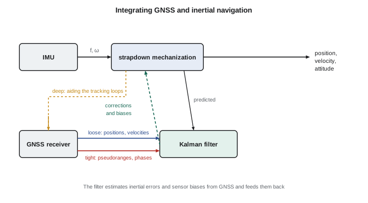
In loosely coupled integration, the GNSS receiver computes its own positions and velocities, and the filter uses them as measurements to correct the inertial solution. It is simple and modular, but it needs a complete GNSS solution, which requires at least four satellites. In tightly coupled integration, the filter uses the raw pseudoranges and carrier phases directly, so even two or three satellites contribute; this helps greatly in partly obstructed environments such as tree-lined roads and urban streets. In deeply or ultra-tightly coupled systems the inertial solution aids the receiver's tracking loops, letting them hold lock on weaker signals. Survey-grade mobile mapping systems normally use tight coupling with carrier-phase ambiguity resolution.
A one-dimensional example
The program below shows the essential behavior with a filter in one dimension. A vehicle moves along a straight road with gently varying speed. An accelerometer with a 0.02 m/s² bias and noise drives the prediction at 10 Hz, and RTK positions with 2 cm noise update the filter once a second. The state contains position, velocity and the accelerometer bias. Between 60 and 90 s there is no GNSS, as under a long overpass.
# A one-dimensional loosely coupled INS/GNSS Kalman filter with a 30 s GNSS outage
import random, math
random.seed(5)

dt = 0.1                                  # IMU rate 10 Hz
bias_true = 0.02                          # accelerometer bias, m/s^2
acc_noise = 0.01                          # accelerometer white noise per sample, m/s^2
gnss_sigma = 0.02                         # RTK position noise, m
outage = (60.0, 90.0)                     # seconds with no GNSS (an underpass on the survey route)

x = [0.0, 0.0, 0.0]                       # estimate: position, velocity, accelerometer bias
P = [[1.0, 0, 0], [0, 1.0, 0], [0, 0, 0.01]]
q_acc, q_bias = acc_noise ** 2, 1e-8
pos = vel = 0.0
def matmul(A, B): return [[sum(A[i][k] * B[k][j] for k in range(len(B))) for j in range(len(B[0]))] for i in range(len(A))]
def T(A): return [list(r) for r in zip(*A)]
F = [[1, dt, -0.5 * dt * dt], [0, 1, -dt], [0, 0, 1]]
Qn = [[0.25 * dt ** 4 * q_acc, 0.5 * dt ** 3 * q_acc, 0], [0.5 * dt ** 3 * q_acc, dt * dt * q_acc, 0], [0, 0, q_bias * dt]]
report = {}
for k in range(1, 1201):
    t = k * dt
    a_true = 0.3 * math.sin(0.05 * t)                       # gentle speed changes of the vehicle
    pos += vel * dt + 0.5 * a_true * dt * dt; vel += a_true * dt
    a_meas = a_true + bias_true + random.gauss(0, acc_noise)
    # predict with the measured acceleration minus the estimated bias
    a_c = a_meas - x[2]
    x = [x[0] + x[1] * dt + 0.5 * a_c * dt * dt, x[1] + a_c * dt, x[2]]
    P = [[a + b for a, b in zip(r1, r2)] for r1, r2 in zip(matmul(matmul(F, P), T(F)), Qn)]
    gnss_ok = not (outage[0] <= t < outage[1])
    if gnss_ok and k % 10 == 0:                              # 1 Hz GNSS position update
        z = pos + random.gauss(0, gnss_sigma)
        S = P[0][0] + gnss_sigma ** 2
        K = [P[i][0] / S for i in range(3)]
        innov = z - x[0]
        x = [x[i] + K[i] * innov for i in range(3)]
        P = [[P[i][j] - K[i] * P[0][j] for j in range(3)] for i in range(3)]
    if k % 50 == 0:
        report[round(t)] = (x[0] - pos, math.sqrt(P[0][0]), x[2])
for t in (10, 30, 60, 65, 70, 75, 80, 85, 90, 95, 120):
    err, sig, b = report[t]
    print("t =", str(t).rjust(3), "s  position error", format(100 * err, "7.1f"), "cm  filter sigma", format(100 * sig, "6.1f"), "cm  bias estimate", format(b, "6.4f"), "m/s^2")
# Unaided drift for comparison: a 0.02 m/s^2 bias over 30 s
print("free-inertial drift from an uncorrected 0.02 m/s^2 bias over 30 s:", round(0.5 * 0.02 * 30 ** 2, 1), "m")t = 10 s position error 0.3 cm filter sigma 1.6 cm bias estimate 0.0207 m/s^2 t = 30 s position error -0.3 cm filter sigma 1.4 cm bias estimate 0.0199 m/s^2 t = 60 s position error 0.4 cm filter sigma 1.8 cm bias estimate 0.0199 m/s^2 t = 65 s position error -5.4 cm filter sigma 5.7 cm bias estimate 0.0199 m/s^2 t = 70 s position error -16.0 cm filter sigma 11.4 cm bias estimate 0.0199 m/s^2 t = 75 s position error -28.5 cm filter sigma 18.9 cm bias estimate 0.0199 m/s^2 t = 80 s position error -42.4 cm filter sigma 28.2 cm bias estimate 0.0199 m/s^2 t = 85 s position error -53.4 cm filter sigma 39.2 cm bias estimate 0.0199 m/s^2 t = 90 s position error 0.9 cm filter sigma 2.0 cm bias estimate 0.0193 m/s^2 t = 95 s position error -1.4 cm filter sigma 1.4 cm bias estimate 0.0198 m/s^2 t = 120 s position error 0.9 cm filter sigma 1.3 cm bias estimate 0.0195 m/s^2 free-inertial drift from an uncorrected 0.02 m/s^2 bias over 30 s: 9.0 m
Within ten seconds the filter has estimated the bias to within about 1 mm/s², and by 30 s almost exactly, because the GNSS updates expose the drift it causes. While GNSS is available the position error stays at about a centimeter. During the outage, the corrected inertial solution drifts slowly, reaching about half a meter after 25 s, whereas an uncorrected bias of the same size would have produced 9 m in 30 s. The filter's own uncertainty grows in step with the actual error, which is what allows downstream processing to know which parts of the trajectory are weak. When GNSS returns, the error collapses within one update.
Post-processing and smoothing
For mapping, the trajectory is normally computed after the survey, not in real time. That allows the use of precise orbits or nearby base stations, and, importantly, a forward filter followed by a backward pass, the Rauch–Tung–Striebel smoother, which uses data from after an outage as well as before it. The smoothed error through a gap is much smaller than the real-time error and peaks in the middle of the gap rather than at its end. Good practice for the canal survey was to drive at moderate speed, to stop in open sky for a few minutes before and after the run so that the filter could settle, and to pass known control targets, whose coordinates in the point cloud served as independent checks.
Lever arms, boresight and timing
The GNSS antenna, the IMU and the scanner or camera are at different places on the vehicle. The lever arms between them, measured in the vehicle frame to a few millimeters, must be applied, rotated by the current attitude, to move the trajectory from the antenna to the IMU and from the IMU to the sensor. An attitude error of 0.01° displaces a point 50 m from the scanner by about 9 mm, so the boresight angles between IMU and scanner are calibrated by surveying a test area from several directions. Every data stream must be time-tagged to the same clock, usually GPS time from the receiver's pulse-per-second output; at 40 km/h, a timing error of 1 ms moves points by 1.1 cm.
Other uses
The same principles appear on a smaller scale in modern survey rovers with tilt compensation, which use a small IMU to measure the pole's tilt and heading so that the pole tip can be positioned without leveling the bubble. They appear in machine control on graders and excavators, in drone photogrammetry and lidar, where they reduce the number of ground control points needed, and in hydrographic surveys, where motion sensors measure the heave, pitch and roll of the vessel. In each case the user must check the integration against independent control, because a poorly calibrated lever arm or tilt sensor produces systematic errors that the precision estimates do not reveal.
Common mistakes
MistakeExpecting an IMU to bridge long outages.
InsteadErrors grow with t² from accelerometer biases and t³ from gyroscope biases; bridge seconds to tens of seconds, not minutes.
MistakeIgnoring the innovation sequence.
InsteadLarge innovations indicate bad measurements or a wrong model; monitor and test them.
MistakeUsing loose coupling in heavily obstructed areas.
InsteadTight coupling uses individual satellites when fewer than four are visible.
MistakeMeasuring lever arms carelessly.
InsteadLever arm errors go directly into the trajectory; measure them to millimeters and check them by calibration.
MistakeStarting a mobile survey without an alignment period.
InsteadStop in open sky so the filter can estimate attitude and biases before and after the run.
Summary and key terms
- An IMU measures specific force and angular rate at high rate and is immune to signal blockage and interference.
- Strapdown mechanization integrates gyro rates for attitude and rotated, gravity-corrected accelerations for velocity and position.
- Accelerometer biases cause position errors growing with t²; gyro biases cause errors growing with t³.
- The Kalman filter alternates prediction and update and weighs measurements by their uncertainties.
- Loose coupling uses GNSS positions; tight coupling uses raw observations; deep coupling aids receiver tracking.
- Integrated filters estimate sensor biases from GNSS and bridge short outages; smoothing improves post-processed trajectories.
- Lever arms, boresight angles and time synchronization must be calibrated and checked.
- IMU
- Inertial measurement unit: three accelerometers and three gyroscopes on orthogonal axes.
- Specific force
- The non-gravitational acceleration measured by an accelerometer.
- Mechanization
- The algorithm that integrates inertial measurements into attitude, velocity and position.
- Kalman filter
- A recursive estimator that combines model predictions and measurements according to their uncertainties.
- Innovation
- The difference between a measurement and its value predicted by the filter.
- Tight coupling
- Integration of inertial data with raw GNSS observations rather than GNSS positions.
Practice problems
Work each problem on paper first, then reveal the answer to check.
An accelerometer bias of 0.01 m/s²: what position error after 20 s?
Show answer
½ × 0.01 × 400 = 2 m.
Why does a gyro bias produce an error that grows with t³?
Show answer
The bias tilts the attitude linearly; the tilt mis-resolves gravity into an acceleration that is integrated twice.
What is the Schuler period?
Show answer
About 84 minutes, the period of the oscillation of horizontal inertial errors.
A Kalman filter predicts a position with σ = 0.30 m and receives a measurement with σ = 0.02 m. Which dominates the update?
Show answer
The measurement; the gain is near 1, about 0.996.
At 60 km/h, how far does the vehicle move in 2 ms?
Show answer
16.7 m/s × 0.002 s = 3.3 cm.
Lesson quiz · 5 questions
Score 60% or more to complete this lesson.
Create a free account to save your progress, take quizzes and earn a certificate.