
ENGG-401 · Lesson 4 of 12 · 28 min
Present worth analysis
Present worth analysis converts every cash flow of an alternative into a single equivalent amount at time 0, discounted at the minimum acceptable rate of return. It is the most widely used and theoretically sound method for evaluating engineering investments, and it is the foundation for the other methods in this course. A positive present worth means that the investment earns more than the MARR; a negative one means it earns less. When comparing alternatives, the one with the highest present worth, or the lowest present cost for cost-only alternatives, is preferred. This lesson covers the present worth method, net present value, independent and mutually exclusive alternatives, equal and unequal lives, the least common multiple and study period approaches, future worth, capitalized cost comparisons, payback periods and their limitations, and practical advice for setting up present worth analyses.
The present worth method
The present worth (PW), also called net present value (NPV), of an alternative at interest rate \(i\) is the sum of its cash flows, each discounted to time 0:
where \(CF_t\) is the net cash flow in period \(t\). In practice, the sum is evaluated with the factors of Lesson 3: first costs at time 0 are taken at face value; uniform series use \((P/A)\); gradients use \((P/G)\) or the geometric formula; single future amounts such as salvage values use \((P/F)\). The interest rate is the MARR. The decision rule for a single investment is simple: accept it if \(PW \ge 0\), because it then recovers its investment and earns at least the MARR; reject it if \(PW < 0\).
Worked problem
Evaluating a single investment
The inspection system from Lesson 1 costs $80,000, saves $22,000 a year for six years and has a $10,000 salvage value. At a MARR of 10 %, should it be purchased?
Show solution
- Savings: \(22{,}000\,(P/A, 10\,\%, 6) = 22{,}000 \times 4.3553 = 95{,}816\).
- Salvage: \(10{,}000\,(P/F, 10\,\%, 6) = 10{,}000 \times 0.5645 = 5{,}645\).
- \(PW = -80{,}000 + 95{,}816 + 5{,}645 = 21{,}460\).
- Because \(PW > 0\), the investment earns more than 10 %.
Answer: PW ≈ +$21,460, so the system should be purchased.
Interpreting present worth
A positive present worth is the amount by which the investment exceeds the MARR in present value terms. If the firm could borrow at the MARR, it could borrow $80,000 plus $21,460, use $80,000 to buy the system, and repay the entire loan from the system's cash flows, keeping $21,460 today. Present worth is therefore a direct measure of the value an investment adds to the firm. It also has the useful property of additivity: the present worth of a group of independent projects is the sum of their individual present worths, which makes it ideal for portfolio decisions.
Independent and mutually exclusive alternatives
Engineering decisions involve two kinds of choice. Independent projects can be accepted or rejected individually: a company might accept every cost-saving project with positive present worth, subject to its budget. Mutually exclusive alternatives meet the same need, so only one can be chosen: a bridge can be built in steel or concrete, not both. For mutually exclusive alternatives, the rule is to choose the alternative with the highest present worth, including the do-nothing alternative with \(PW = 0\) if it is feasible. When the alternatives have only costs, such as different pumps for the same duty with equal benefits, it is convenient to treat costs as positive and choose the alternative with the lowest present cost. Sometimes one alternative must be chosen even if all have negative present worth, for example when a regulation requires treatment of wastewater; then the least negative present worth is best.
Equal-life alternatives
When mutually exclusive alternatives have the same life, present worths over that life can be compared directly.
Worked problem
Comparing two pumps
Pump A costs $50,000, has annual operating and maintenance costs of $9,000 and a salvage value of $5,000 after 10 years. Pump B costs $70,000, has annual costs of $6,000 and a salvage value of $10,000 after 10 years. Both deliver the same service. At a MARR of 10 %, which is preferred?
Show solution
- Factors at 10 %, 10 years: \((P/A) = 6.1446\), \((P/F) = 0.3855\).
- Pump A: \(PW = -50{,}000 - 9{,}000 \times 6.1446 + 5{,}000 \times 0.3855 = -103{,}373\).
- Pump B: \(PW = -70{,}000 - 6{,}000 \times 6.1446 + 10{,}000 \times 0.3855 = -103{,}012\).
- Pump B has the slightly smaller present cost, by about $360.
Answer: Pump B is marginally preferred, but the difference is so small that non-monetary factors, risk or a sensitivity analysis should guide the final choice.
The example illustrates an important practical point: when present worths are within the uncertainty of the estimates, the analysis does not clearly favor either alternative, and the decision should consider reliability, energy price risk, maintenance support and other factors. Lesson 12 explores this with sensitivity analysis.
Unequal lives: least common multiple
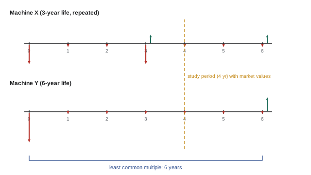
Present worths of alternatives with different lives cannot be compared directly, because they cover different periods of service. One approach assumes that each alternative is repeated with identical cash flows until all reach the end of a common period, the least common multiple (LCM) of their lives. An alternative with a 3-year life and one with a 6-year life are compared over 6 years, with the first repeated twice.
Worked problem
Least common multiple comparison
Machine X costs $30,000, has annual costs of $5,000, a 3-year life and a $3,000 salvage value. Machine Y costs $45,000, has annual costs of $3,500, a 6-year life and a $5,000 salvage value. At a MARR of 12 %, which is cheaper?
Show solution
- One cycle of X: \(PW = -30{,}000 - 5{,}000 \times 2.4018 + 3{,}000 \times 0.7118 = -39{,}874\).
- Two cycles of X over 6 years: \(-39{,}874 - 39{,}874 \times (P/F, 12\,\%, 3) = -39{,}874 - 39{,}874 \times 0.7118 = -68{,}255\).
- Machine Y over 6 years: \(-45{,}000 - 3{,}500 \times 4.1114 + 5{,}000 \times 0.5066 = -56{,}857\).
- Y has the lower present cost over the common 6-year period.
Answer: Machine Y is preferred, with a present cost about $11,400 lower over six years.
The LCM approach assumes that future replacements will have identical costs and that the service is needed for the whole period. These assumptions may be unrealistic, particularly with rapid technological change or when the LCM is very long; lives of 7 and 9 years have an LCM of 63 years. Annual worth analysis (Lesson 5) handles unequal lives more conveniently under the same assumptions.
Unequal lives: study period
The study period approach compares alternatives over a fixed planning horizon chosen to reflect how long the service is actually needed, often shorter than the longest life. Cash flows beyond the study period are ignored, and each alternative is credited with an estimated market value of its assets at the end of the study period. For example, if a contractor needs equipment only for a 4-year project, alternatives are compared over 4 years with estimated resale values at year 4, whatever their physical lives. The study period approach is often more realistic than the LCM approach but requires estimates of future market values, which may be uncertain.
Future worth
Future worth (FW) analysis moves all cash flows to the end of the study period instead of the beginning. Because \(FW = PW\,(F/P, i, n)\), it always leads to the same decision as present worth. Future worth is useful when decision-makers think in terms of the value at a future date, for example the accumulated value of a construction project at completion, or the value of an investment when a facility comes into service. For the inspection system, \(FW = 21{,}460 \times 1.7716 = 38{,}019\) at year 6.
Capitalized cost comparisons
For long-lived public works, alternatives can be compared by capitalized cost, the present worth of providing the service forever (Lesson 3). For example, a tunnel lining with a 50-year life might be compared with one lasting 100 years by converting each lining's first cost into an equivalent perpetual annual cost with \((A/P, i, n)\), adding annual maintenance, and dividing by \(i\). Capitalized cost is effectively a present worth comparison with an infinite study period and repeated replacements.
Payback period
The payback period is the time required for cumulative net cash flows to recover the initial investment. Simple payback ignores the time value of money; for the inspection system, simple payback is \(80{,}000 / 22{,}000 = 3.6\) years. Discounted payback uses discounted cash flows and is longer; at 10 %, the cumulative discounted cash flow turns positive between years 4 and 5, at about 4.8 years. Payback is popular because it is easy to understand and indicates how quickly capital is returned, which matters for liquidity and risk, especially with uncertain technology. But it has serious flaws as a decision criterion: it ignores cash flows after the payback point, so it can favor a project that pays back quickly but earns little over one with a slightly longer payback and much larger long-term benefits, and simple payback ignores the time value of money altogether. Payback is best used as a supplementary indicator alongside present worth, not as the primary criterion.
| Year | Net cash flow | Discounted at 10 % | Cumulative discounted |
|---|---|---|---|
| 0 | −80,000 | −80,000 | −80,000 |
| 1 | 22,000 | 20,000 | −60,000 |
| 2 | 22,000 | 18,182 | −41,818 |
| 3 | 22,000 | 16,529 | −25,289 |
| 4 | 22,000 | 15,026 | −10,263 |
| 5 | 22,000 | 13,660 | 3,397 |
| 6 | 32,000 | 18,063 | 21,460 |
Setting up present worth analyses
Good practice in present worth analysis includes:
- Drawing a cash flow diagram for each alternative, from the same point of view.
- Including only cash flows that differ between alternatives, and including the do-nothing alternative where feasible.
- Using a consistent study period for mutually exclusive alternatives.
- Using the MARR appropriate to the project's risk.
- Treating inflation consistently, using either real cash flows with a real interest rate or nominal cash flows with a nominal rate (Lesson 10).
- Including taxes where relevant, using after-tax cash flows and an after-tax MARR (Lesson 9).
- Presenting results with a sensitivity analysis showing how present worth changes with key estimates.
Present worth of life-cycle costs for buildings
Life-cycle cost analysis (LCCA) applies present worth to building systems, where operating costs over decades often exceed the first cost many times. A high-performance envelope, triple-glazed windows or a ground-source heat pump may cost more to build but less to operate. LCCA guidelines for public buildings in both countries specify study periods (often 25 to 40 years), discount rates, energy price escalation and replacement cycles for components with shorter lives, such as roofs, boilers and lighting. Residual values for components with remaining life at the end of the study period are credited. Because energy prices and discount rates strongly affect results, LCCA reports typically include sensitivity analyses of both.
Present worth and project finance
In project finance, present worth is calculated for the whole project and separately for lenders and equity investors. Lenders care about whether cash flows can cover debt service with a margin, measured by the debt service coverage ratio, while equity investors care about the present worth and IRR of their own cash flows after debt payments. Engineers preparing technical inputs for project finance should understand these perspectives.
Choosing the study period
Selecting the study period is an important judgment. It should reflect the period over which the service is needed and over which estimates are meaningful; very long periods add little because distant cash flows are heavily discounted, but they matter for public infrastructure with low discount rates.
Common mistakes
MistakeComparing present worths over different lives.
InsteadUse the LCM, a study period or annual worth.
MistakeChoosing by payback period alone.
InsteadUse present worth as the primary criterion.
MistakeIgnoring salvage values.
InsteadInclude salvage or market value at the end of the period.
MistakeTreating small PW differences as decisive.
InsteadCompare with estimate uncertainty and other factors.
MistakeMixing costs as positive and negative inconsistently.
InsteadUse one sign convention for all alternatives.
Summary and key terms
- Present worth discounts all cash flows to time 0 at the MARR.
- Accept a single investment if PW ≥ 0.
- PW measures the value an investment adds and is additive across projects.
- Choose the mutually exclusive alternative with the highest PW or lowest present cost.
- Unequal lives require an LCM, a study period or annual worth.
- Future worth gives the same decision as present worth.
- Payback is a supplementary indicator; it ignores later cash flows.
- Present worth
- Equivalent value of all cash flows at time 0.
- Net present value
- Another name for present worth.
- Independent projects
- Projects that can be accepted individually.
- Mutually exclusive alternatives
- Alternatives of which only one can be chosen.
- Present cost
- Present worth of costs treated as positive.
- Least common multiple
- Common period for repeated alternatives.
- Study period
- Fixed planning horizon for comparison.
- Future worth
- Equivalent value at the end of the study period.
- Simple payback
- Time to recover investment ignoring interest.
- Discounted payback
- Time to recover investment with discounting.
Practice problems
Work each problem on paper first, then reveal the answer to check.
PW of a $10,000 investment returning $3,000 a year for 5 years at 10 %?
Show answer
About +$1,372.
What does a positive PW mean?
Show answer
The investment earns more than the MARR.
Decision rule for mutually exclusive alternatives?
Show answer
Choose the highest PW, including do-nothing if feasible.
LCM of lives 4 and 6 years?
Show answer
12 years.
What assumption does the LCM approach make?
Show answer
Identical repeated cycles and need for the whole period.
What does the study period approach need?
Show answer
Market values at the end of the period.
Relationship between FW and PW?
Show answer
FW = PW (F/P, i, n).
Simple payback of $50,000 with $12,500 a year?
Show answer
4 years.
Main flaw of payback?
Show answer
Ignores cash flows after payback.
Why is PW additive useful?
Show answer
Portfolio PW is the sum of project PWs.
Lesson quiz · 5 questions
Score 60% or more to complete this lesson.
Create a free account to save your progress, take quizzes and earn a certificate.