Converter dynamics and control

A converter that delivers exactly 12 V at full load in a steady-state calculation is only half designed. In service, its input voltage varies, its load jumps from idle to full power in microseconds when a processor wakes up, and its components drift with temperature and age. Feedback control keeps the output where it should be through all of this, and its design decides whether the output recovers cleanly from a disturbance or rings, overshoots or oscillates. Lesson 5 introduced voltage-mode and current-mode control in a paragraph. This lesson develops the tools behind them: averaged models that make switching converters look like ordinary linear systems, the transfer functions of the buck and boost converters, the design of compensators using loop gain, phase margin and crossover frequency, the advantages of current-mode control, the simulation of load transients, and the digital controllers that now implement most loops.

Averaging the switching

A switching converter is a nonlinear, time-varying circuit: its topology changes twice in every switching period. For control design, what matters is how the average voltages and currents change over many periods, not the ripple within each one. State-space averaging replaces the switched circuit with a continuous model whose equations are the duty-cycle-weighted average of the equations for each switch position. For a buck converter in continuous conduction, with inductor current \(i_L\) and capacitor voltage \(v_C\):

where \(d\) is the duty cycle. This averaged model is valid for frequencies well below the switching frequency. Linearizing it around an operating point (small perturbations in duty cycle, input voltage and load) gives transfer functions that describe how the output responds to each.

Transfer functions of basic converters

For the buck converter, the control-to-output transfer function, from small changes in duty cycle to small changes in output voltage, is that of a second-order low-pass filter scaled by the input voltage, with a zero from the capacitor's ESR:

It has a double pole at the resonant frequency \(f_0 = 1/(2\pi\sqrt{LC})\), where the gain peaks by an amount set by the quality factor \(Q = R\sqrt{C/L}\) and the phase drops rapidly by 180 degrees. Above \(f_0\) the gain falls at 40 dB per decade until the ESR zero, where it flattens to 20 dB per decade. A light load (large \(R\)) gives a high \(Q\) and a sharp resonant peak.

The boost converter is harder to control. Its averaged model has the same double pole, but also a right-half-plane zero at \(f_{RHP} = R(1-D)^2/(2\pi L)\). A right-half-plane zero adds gain like an ordinary zero but subtracts phase like a pole, and physically reflects the fact that increasing the duty cycle first reduces the energy delivered to the output (the switch is on longer, so the inductor is connected to the output for less time) before the inductor current rises and output increases. The control loop must cross over well below this zero, typically at a fifth of its frequency or less, which limits how fast a boost converter can respond. The flyback and buck-boost converters share this limitation.

Loop gain, crossover and phase margin

In a voltage-mode controller, the output is compared with a reference, the error is processed by a compensator \(G_c(s)\), and the result sets the duty cycle through a pulse-width modulator with gain \(1/V_{ramp}\). The loop gain \(T(s)\) is the product of all the transfer functions around the loop. Its frequency response, shown on a Bode plot, determines the closed-loop behavior:

• The crossover frequency \(f_c\), where \(|T| = 1\) (0 dB), sets the bandwidth: the loop corrects disturbances slower than \(f_c\) and ignores faster ones. A common target is a tenth to a fifth of the switching frequency.
• The phase margin, 180 degrees plus the phase of \(T\) at crossover, measures how far the loop is from oscillating. Values of 45 to 70 degrees give well-damped responses; low margins produce ringing and overshoot.
• The gain margin, how far \(|T|\) is below 0 dB where the phase reaches -180 degrees, measures robustness to gain variations.
• High gain at low frequency, usually from an integrator, eliminates steady-state error.

Because the buck's double pole removes 180 degrees of phase, a simple integrator or proportional-integral controller crossing over above \(f_0\) would leave almost no phase margin. Voltage-mode controllers therefore use a type III compensator: an integrator, two zeros placed near the double pole to restore phase, and two poles at higher frequency (near the ESR zero and half the switching frequency) to attenuate switching noise.

import numpy as np

# Small-signal control-to-output transfer function of a buck converter, and a type III compensator
Vin, L, C, Resr, R = 48.0, 10e-6, 200e-6, 0.005, 1.2
Vramp = 1.0                                         # PWM ramp amplitude, V

def Gvd(f):
    s = 2j * np.pi * f
    Zc = Resr + 1 / (s * C)
    Zload = Zc * R / (Zc + R)
    return Vin / Vramp * Zload / (Zload + s * L)    # duty to output voltage

f0 = 1 / (2 * np.pi * np.sqrt(L * C))
print(f"LC double pole at {f0 / 1e3:.2f} kHz, Q = {R * np.sqrt(C / L):.1f}, ESR zero at {1 / (2 * np.pi * Resr * C) / 1e3:.0f} kHz")

wz, wp = 2 * np.pi * 3e3, 2 * np.pi * 100e3
def Gc(f, K):
    s = 2j * np.pi * f
    return K * (1 + s / wz) ** 2 / (s * (1 + s / wp) ** 2)

fc = 20e3                                           # target crossover frequency
K = 1 / abs(Gvd(fc) * Gc(fc, 1.0))
f = np.logspace(2, 5.5, 4000)
T = Gvd(f) * Gc(f, K)
i_c = np.argmin(abs(abs(T) - 1))
pm = 180 + np.degrees(np.angle(T[i_c]))
ph = np.unwrap(np.angle(T))
i_180 = np.argmin(abs(np.degrees(ph) + 180))
gm = -20 * np.log10(abs(T[i_180]))
print(f"compensator gain K = {K:.0f}; crossover {f[i_c] / 1e3:.1f} kHz, phase margin {pm:.0f} deg, gain margin {gm:.0f} dB")
for fx in (300, 1e3, 3.56e3, 10e3, 20e3, 50e3):
    g = Gvd(fx)
    t = g * Gc(fx, K)
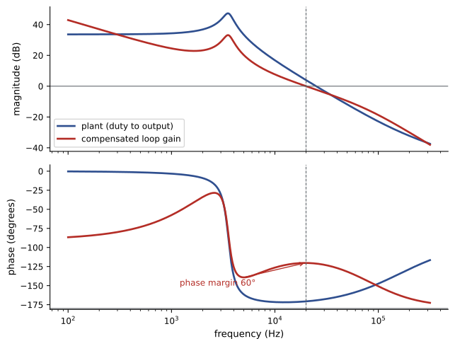
    print(f"{fx / 1e3:6.2f} kHz: plant {20 * np.log10(abs(g)):6.1f} dB {np.degrees(np.angle(g)):7.1f} deg | loop {20 * np.log10(abs(t)):6.1f} dB")

LC double pole at 3.56 kHz, Q = 5.4, ESR zero at 159 kHz
compensator gain K = 1827; crossover 20.0 kHz, phase margin 60 deg, gain margin 38 dB
  0.30 kHz: plant   33.7 dB    -0.9 deg | loop   33.5 dB
  1.00 kHz: plant   34.3 dB    -3.3 deg | loop   24.5 dB
  3.56 kHz: plant   47.2 dB   -90.0 deg | loop   33.1 dB
 10.00 kHz: plant   16.8 dB  -171.6 deg | loop    7.6 dB
 20.00 kHz: plant    3.9 dB  -170.7 deg | loop   -0.0 dB
 50.00 kHz: plant  -11.9 dB  -161.7 deg | loop   -9.6 dB

The plant's gain peaks by about 13 dB at the 3.6 kHz resonance, and its phase falls to about -170 degrees above it. The compensator's zeros at 3 kHz restore phase so that the loop crosses over at 20 kHz, a tenth of the 200 kHz switching frequency, with 60 degrees of phase margin and a large gain margin. Designers verify such calculations by measuring the loop gain of the actual converter with a network analyzer, injecting a small signal into the loop, because parasitic elements and component tolerances shift the real response.

Current-mode control

Current-mode control adds an inner loop that controls the inductor current directly. In peak current-mode control, the switch turns on at the start of each period and turns off when the sensed inductor current reaches a threshold set by the outer voltage loop. The inner loop effectively turns the inductor into a controlled current source, removing one of the two poles of the LC filter from the outer loop. The voltage loop then sees a first-order system, the output capacitor and load, which a simple proportional-integral (type II) compensator can control with good phase margin.

Current-mode control has further advantages. It limits the switch current on every cycle, providing fast protection against overloads and short circuits. It rejects input voltage changes quickly, because a higher input voltage makes the current ramp faster and reach the threshold sooner. And it allows parallel converters to share current, because each converter's current follows the same control signal. Its main complication is subharmonic oscillation: in peak current mode with duty cycles above 50 percent, small disturbances in inductor current grow from cycle to cycle unless a compensating ramp, with a slope of at least half the inductor current's down-slope, is added to the sensed current. Average current-mode control, which uses a compensated amplifier on the averaged inductor current, avoids this and is common in power factor correction circuits.

Load transients

For many loads, the most demanding test is a load step: a processor or memory changing from idle to full load in a microsecond or less. Until the control loop responds, the extra current must come from the output capacitor, so the output voltage dips. The size of the dip depends on how much charge the capacitor supplies before the inductor current catches up, which depends on the loop bandwidth, the inductor's slew rate (limited by \(V_{in} - V_{out}\) across \(L\)), and the capacitor's ESR and ESL, which cause an immediate step in voltage.

import numpy as np

# Averaged simulation of a 48 V to 12 V buck with current-mode inner loop and PI voltage loop: load step 5 A to 15 A
Vin, L, C, Vref = 48.0, 10e-6, 200e-6, 12.0
dt, Ts = 0.05e-6, 5e-6                       # integration step and control period (200 kHz)

def run(kp, ki, steps=int(2.0e-3 / 0.05e-6)):
    iL, v, integ, d = 5.0, 12.0, 5.0, 0.25
    vmin, t_settle = 99.0, None
    for n in range(steps):
        t = n * dt
        I_load = 5.0 if t < 0.2e-3 else 15.0
        if n % int(Ts / dt) == 0:            # controller update once per switching period
            e = Vref - v
            integ += ki * e * Ts
            i_ref = np.clip(kp * e + integ, 0, 30)
            d = np.clip((v + 3.0 * (i_ref - iL)) / Vin, 0, 0.95)   # inner current loop, gain 3 V/A
        iL += (d * Vin - v) / L * dt
        v += (iL - I_load) / C * dt
        if t > 0.2e-3:
            vmin = min(vmin, v)
            if abs(v - Vref) > 0.12:
                t_settle = None
            elif t_settle is None:
                t_settle = t - 0.2e-3
    return vmin, t_settle

for label, kp, ki in (("slow voltage loop", 3.0, 1e4), ("faster voltage loop", 15.0, 2.25e5)):
    vmin, ts = run(kp, ki)
    tstxt = f"{ts * 1e6:.0f} us" if ts is not None else "not settled"
    print(f"{label}: minimum {vmin:.3f} V (dip {12 - vmin:.3f} V), back within 1% after {tstxt}")

slow voltage loop: minimum 9.475 V (dip 2.525 V), back within 1% after 886 us
faster voltage loop: minimum 11.458 V (dip 0.542 V), back within 1% after 117 us

The faster voltage loop limits the dip to about half a volt and recovers within about 120 µs, while the slow loop lets the output fall by more than 2.5 V. Even the faster result, a 4.5 percent dip, would be too much for a processor, whose supply must typically stay within a few percent. Processor power supplies, called voltage regulators, therefore combine very fast control (often with crossover frequencies above 100 kHz, multiphase converters running at high effective frequency, and nonlinear responses that turn on all phases at once when a step is detected), large banks of low-ESR ceramic and polymer capacitors close to the processor, and adaptive voltage positioning, in which the output is deliberately allowed to droop with load so that transients use the whole tolerance band.

Input filters and negative resistance

A converter with a tightly regulated output draws constant power from its input. If the input voltage rises, the input current falls, and vice versa: within the control bandwidth, the converter looks like a negative incremental resistance to its source. When the source is an LC input filter (needed to meet EMI limits, Lesson 8) or a long cable, this negative resistance can cancel the filter's damping and cause oscillation. Middlebrook's criterion, published in 1976, states that the output impedance of the input filter must be much smaller than the converter's input impedance at all frequencies. Designers meet it by adding damping to the filter, typically a resistor in series with a capacitor across the filter capacitor. The same instability appears in DC distribution systems with many tightly regulated loads, such as aircraft, ships, electric vehicles and data center DC buses.

Digital control

Most modern converters above a few hundred watts, and many smaller ones, use digital control. A microcontroller or dedicated controller samples the output voltage and inductor current with analog-to-digital converters, computes the compensator as a difference equation, and sets the duty cycle with a high-resolution digital pulse-width modulator. Digital control introduces delays (sampling, computation and the modulator's update) that erode phase margin, and quantization of both measurements and duty cycle, which can cause small limit-cycle oscillations if the duty cycle resolution is too coarse; designers account for these in the loop design.

In return, digital control allows nonlinear and adaptive strategies, automatic tuning, digital telemetry over the PMBus interface, fault logging, coordination of many phases, and different modes for light and heavy load to keep efficiency high across the range. Complex converters, such as three-phase active front ends, grid-connected inverters (Lesson 7) and motor drives (Lesson 9), use digital control with transformations into rotating reference frames, as described in those lessons.