
ELE-240 · Lesson 12 of 12 · 23 min
Frequency response basics and an amplifier design project
Every amplifier calculation so far has assumed mid-band frequencies, where coupling and bypass capacitors are short circuits and the transistor's own capacitances are open circuits. Neither assumption holds at all frequencies. At low frequencies the external capacitors' reactance grows until they no longer pass the signal, and the gain falls. At high frequencies the tiny internal capacitances of the transistor start to conduct signal current, and the gain falls again. The range between, where the gain is flat, is the amplifier's bandwidth. This lesson introduces the tools for estimating both corners, and then walks through the complete design of the microphone amplifier as a project, from specification to bench test. ELE-340 treats frequency response in full; the goal here is good first estimates.
Bode plots and decibels
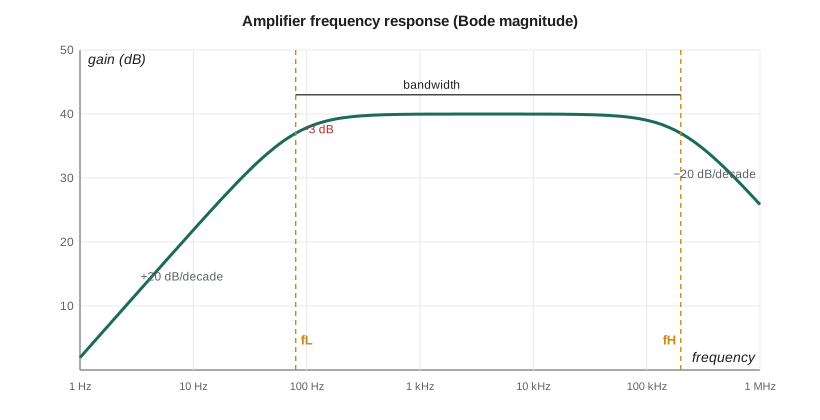
Frequency response is plotted on a Bode plot: gain in decibels against frequency on a logarithmic scale. The decibel converts ratios into sums: a voltage gain A is 20 log₁₀|A| dB, so a gain of 10 is 20 dB, 100 is 40 dB and 1,000 is 60 dB, while halving the power, a gain of 1/√2 in voltage, is −3 dB. A single RC network gives a corner, or pole, at f = 1/(2πRC). Beyond the corner, the gain changes by 20 dB per decade of frequency, and at the corner itself it is 3 dB below its mid-band value. The bandwidth of an amplifier is usually defined between its two −3 dB frequencies, f_L and f_H.
Low-frequency response: coupling and bypass capacitors
Each coupling or bypass capacitor forms a high-pass network with the resistance it sees. A useful estimate, the short-circuit time-constant method, treats each capacitor alone: with all other capacitors shorted and signal sources set to zero, find the resistance R_k seen by capacitor C_k, and add up the corner frequencies:
For an input coupling capacitor the resistance is R_sig + R_in; for an output coupling capacitor it is R_out + R_L. The emitter bypass capacitor is usually the troublemaker, because looking into the emitter it sees a very low resistance: R_E2 in parallel with r_e plus any unbypassed resistance plus the source resistance divided by β + 1. With such a small resistance, a bypass capacitor needs to be far larger than the coupling capacitors to give the same corner. Designers usually pick the bypass capacitor to set f_L and make the coupling capacitors' corners several times lower, so they do not add much.
Worked problem
Choosing capacitors for a 100 Hz low corner
In the first stage of the microphone amplifier, the input capacitor sees R_sig + R_in = 2 kΩ + 12 kΩ = 14 kΩ, the output capacitor sees 4.7 kΩ + 15 kΩ ≈ 20 kΩ, and the bypass capacitor across R_E2 sees about R_E2 ∥ (r_e + R_E1 + (R_sig ∥ R_B)/(β + 1)) ≈ 1.4 kΩ ∥ (28 + 100 + 11) ≈ 126 Ω. Choose capacitors for f_L ≈ 100 Hz, with the bypass capacitor setting the corner.
Show solution
- Let the bypass capacitor contribute about 80 Hz:
- \[C_E = \frac{1}{2\pi \times 126 \times 80} \approx 15.8\ \mu\text{F} \to 22\ \mu\text{F}\;(f \approx 57\ \text{Hz})\]
- Let each coupling capacitor contribute about 10 Hz or less:
- \[C_{in} \ge \frac{1}{2\pi \times 14\,000 \times 10} \approx 1.1\ \mu\text{F} \to 2.2\ \mu\text{F}\;(5\ \text{Hz}), \qquad C_{out} \to 1\ \mu\text{F}\;(8\ \text{Hz})\]
- \[f_L \approx 57 + 5 + 8 \approx 70\ \text{Hz}\]
Answer: With 22 µF, 2.2 µF and 1 µF, the estimated low corner is about 70 Hz, below the 100 Hz target, which leaves room for capacitor tolerance; electrolytic capacitors are often −20 percent or worse.
High-frequency response: the transistor's capacitances
Inside the transistor, the junctions store charge. In the hybrid-π model this appears as a capacitance C_π from base to emitter, mostly the diffusion capacitance of the forward-biased junction, and a smaller capacitance C_μ from base to collector, the depletion capacitance of the reverse-biased junction, typically a few picofarads for a small transistor. MOSFETs have the corresponding C_gs and C_gd. A transistor's speed is summarized by its transition frequency f_T, the frequency at which its short-circuit current gain falls to 1:
For a 2N3904-class part, f_T is about 300 MHz at a few milliamps, falling at lower currents because g_m falls. A transistor is not much use as an amplifier much above f_T divided by the gain required.
The Miller effect
In a common-emitter stage, C_μ connects the input to the inverted output. When the base rises by a small voltage v, the collector falls by A v, so the voltage across C_μ changes by (1 + |A|)v, and it draws (1 + |A|) times the current a grounded capacitor would. Seen from the input, C_μ behaves like a capacitance multiplied by the gain, the Miller effect:
Here R_sig' is the source resistance in parallel with the bias network and r_π' is the resistance looking into the base. Because the gain multiplies C_μ, a high-gain CE stage driven from a high source resistance has a surprisingly low upper corner. This is why the common-base stage, which has no Miller multiplication, and the cascode, which holds the CE transistor's collector nearly still, are used in wideband amplifiers. It is also why emitter degeneration widens bandwidth: lower gain means a smaller Miller capacitance.
Worked problem
Upper corner of the first stage
The first stage has C_π = 18 pF and C_μ = 4 pF at its bias point, a gain from base to collector of about −12, and a resistance at the base node of about R_sig ∥ R_B ∥ r_π' = 2 kΩ ∥ 15 kΩ ∥ 19 kΩ ≈ 1.6 kΩ. With degeneration, the effective C_π is reduced by roughly 1 + g_m R_E1 ≈ 4.6. Estimate f_H.
Show solution
- \[C_{in} \approx \frac{18}{4.6} + 4(1 + 12) \approx 3.9 + 52 \approx 56\ \text{pF}\]
- \[f_H \approx \frac{1}{2\pi \times 1600 \times 56 \times 10^{-12}} \approx 1.8\ \text{MHz}\]
Answer: The input pole is near 1.8 MHz, so the Miller capacitance dominates but is no limitation for a voice-band amplifier; wiring capacitance and the following stage's input will set the real upper corner. Amara will deliberately add a small capacitor across R_C to roll the gain off above about 10 kHz and reject radio-frequency pickup from nearby transmitters.
import math
# Bode magnitude of the two-stage microphone amplifier from its corner frequencies
AM = 100.0                     # mid-band gain
lows = [57.0, 5.0, 8.0, 57.0, 5.0, 8.0]   # capacitor corners of both stages, Hz
highs = [10e3, 1.8e6]          # deliberate roll-off and Miller pole, Hz
def gain(f):
    g = AM
    for fl in lows:
        g *= (f / fl) / math.sqrt(1 + (f / fl) ** 2)
    for fh in highs:
        g /= math.sqrt(1 + (f / fh) ** 2)
    return g
for f in (20, 50, 100, 200, 500, 1000, 3000, 10000, 30000):
    print(f"{f:6d} Hz: {20 * math.log10(gain(f)):6.1f} dB")
# find the -3 dB points numerically
mid = 20 * math.log10(gain(1000))
def corner(lo, hi, rising):
    for _ in range(60):
        m = math.sqrt(lo * hi)
        above = 20 * math.log10(gain(m)) > mid - 3
        if above == rising: hi = m
        else: lo = m
    return m
print(f"fL = {corner(10, 1000, True):.0f} Hz, fH = {corner(1000, 1e6, False)/1000:.1f} kHz") 20 Hz: 19.0 dB
50 Hz: 32.5 dB
100 Hz: 37.5 dB
200 Hz: 39.3 dB
500 Hz: 39.9 dB
1000 Hz: 39.9 dB
3000 Hz: 39.6 dB
10000 Hz: 37.0 dB
30000 Hz: 30.0 dB
fL = 89 Hz, fH = 10.1 kHzThe output shows something the single-stage estimate hid. With two stages, each contributing similar corners, the combined low corner is higher than the 70 Hz of one stage, because the attenuation of the two stages multiplies. The combined corner of about 90 Hz still meets the 150 Hz requirement, so Amara keeps the 22 µF bypass capacitors; doubling them would push it down to about 50 Hz if the specification changed.
The design project: the noise-sensing microphone amplifier
A design project pulls every lesson together. Cedarline's process, like that of most engineering firms, has five stages: specification, architecture, detailed design, verification by analysis and simulation, and bench testing, each documented and reviewed. The microphone amplifier is small enough to follow through all five.
| Requirement | Target | Source of requirement |
|---|---|---|
| Mid-band gain, microphone to detector | ≈ 100 (40 dB) ± 20 % | Detector needs about 0.3 V at typical street noise |
| Low corner f_L | ≤ 150 Hz | Street noise energy is mostly above 100 Hz |
| High corner f_H | ≈ 8 to 12 kHz, then roll off | Speech and traffic band; reject radio pickup |
| Input resistance | ≥ 10 kΩ | Microphone output resistance about 2 kΩ |
| Supply | 12 V rail, < 10 mA | Power budget of the pushbutton station |
| Temperature range | −40 °C to +74 °C | Cabinet and pole-mounted station |
| Gain drift over temperature | < ± 1 dB | Noise-level calibration |
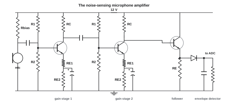
Architecture follows from the specification and lesson 11: two degenerated CE stages for a stable gain near 100, an emitter follower to drive the detector, and the envelope detector itself. Detailed design repeats the steps of the earlier lessons: bias each stage with voltage-divider bias and V_E ≥ 1.4 V; choose R_C/R_E1 for a gain of about −12 per stage after loading; check the input resistance and raise the divider resistors if needed; choose coupling and bypass capacitors for f_L; add the roll-off capacitor for f_H; size the follower's bias for the detector's charging current. The total current is about 0.9 + 0.9 + 2 mA plus divider currents, under 5 mA.
Verification starts with a worst-case analysis: β from 100 to 300, V_BE drift over temperature, resistor tolerances of 1 percent and capacitor tolerances of −20 to +50 percent. Because each stage's gain is about R_C/(r_e + R_E1), and r_e = V_T/I_E changes with temperature and bias, the gain drifts slightly; with R_E1 four times r_e, a 25 percent swing in r_e changes each stage's gain by about 5 percent, and the two stages together by about 10 percent, roughly 0.8 dB, inside the ±1 dB budget. A circuit simulation then checks the DC operating points, the frequency response and the distortion at the largest expected signal, using the transistor manufacturer's models across temperature.
Bench testing closes the loop. Amara builds a prototype, measures the DC voltages at every node against her calculations, sweeps the frequency response with a signal generator and an oscilloscope or audio analyzer, measures distortion at the maximum input, and repeats the key measurements in a temperature chamber at −40 °C and +74 °C. Disagreements between calculation, simulation and measurement are investigated, not ignored: each one is either a modeling error to fix or a real problem in the circuit. Daniel signs off the design review only when the three agree within the expected tolerances, and the records go into the project file that a professional engineer will rely on when the product is certified for use on public roads.
Common mistakes
MistakeForgetting that each extra stage adds its own low and high corners.
InsteadCorners of cascaded stages combine; two similar corners shift the overall −3 dB point.
MistakeSizing the emitter bypass capacitor like a coupling capacitor.
InsteadIt sees only tens to hundreds of ohms and needs a much larger value for the same corner.
MistakeIgnoring the Miller effect in a high-gain CE stage.
InsteadC_μ appears multiplied by (1 + |A|) at the input and often sets f_H.
MistakeTreating a design as finished when the simulation works.
InsteadDo worst-case analysis, then measure the prototype across temperature and reconcile all three.
Summary and key terms
- Bode plots show gain in dB against log frequency; each RC corner changes the slope by 20 dB per decade.
- Coupling and bypass capacitors set f_L; estimate it by summing 1/(2πR_kC_k) for each capacitor.
- The emitter bypass capacitor sees a small resistance and usually sets f_L.
- Transistor capacitances C_π and C_μ set f_H; f_T = g_m/(2π(C_π + C_μ)).
- The Miller effect multiplies C_μ by (1 + |A|); lower gain or a cascode widens bandwidth.
- A design project runs from specification through architecture, detailed design, worst-case verification and bench test.
- Bandwidth
- The frequency range between the lower and upper −3 dB frequencies of an amplifier.
- Decibel
- A logarithmic measure of gain; a voltage gain A is 20 log₁₀|A| dB.
- Pole
- A corner in the frequency response where the slope changes by −20 dB per decade.
- Short-circuit time-constant method
- Estimating f_L by summing the corners of each capacitor taken alone.
- Transition frequency
- f_T, the frequency at which a transistor's short-circuit current gain falls to 1.
- Miller effect
- The multiplication of a feedback capacitance by (1 + |A|) when seen from the input.
- Worst-case analysis
- Checking a design at the extremes of every parameter tolerance and operating condition.
Practice problems
Work each problem on paper first, then reveal the answer to check.
Express a voltage gain of 316 in decibels.
Show answer
20 log₁₀ 316 ≈ 50 dB.
A coupling capacitor of 1 µF sees 16 kΩ. Find its corner frequency.
Show answer
1/(2π × 16 000 × 10⁻⁶) ≈ 10 Hz.
An emitter bypass capacitor sees 30 Ω. What capacitance gives a 50 Hz corner?
Show answer
1/(2π × 30 × 50) ≈ 106 µF.
A transistor has g_m = 40 mS, C_π = 16 pF and C_μ = 4 pF. Find f_T.
Show answer
0.04/(2π × 20 pF) ≈ 318 MHz.
C_μ = 3 pF in a stage with gain −99. What is the Miller capacitance at the input?
Show answer
3 pF × 100 = 300 pF.
Why does emitter degeneration usually increase an amplifier's bandwidth?
Show answer
It lowers the gain and so the Miller multiplication of C_μ, and it reduces the effective C_π.
Lesson quiz · 5 questions
Score 60% or more to complete this lesson.
Create a free account to save your progress, take quizzes and earn a certificate.