
ELE-240 · Lesson 10 of 12 · 24 min
Small-signal models
Transistors are nonlinear: the BJT's collector current depends exponentially on v_BE and the MOSFET's drain current on the square of its overdrive. Yet amplifiers are expected to be linear, so that a voice or a sensor signal comes out larger but with the same shape. The resolution is the small-signal idea. Bias the transistor at a DC operating point, then add a signal small enough that the curve looks straight over the range it covers. For that small signal, the transistor behaves like a linear circuit of resistors and controlled sources, and all the linear circuit tools of ELE-202 apply. This lesson builds those linear models; lesson 11 uses them to design amplifiers.
The accessible pedestrian signal's microphone produces only a few millivolts at normal street noise levels. Amara must amplify that by a factor of about a hundred before the envelope detector from lesson 4 can measure it. To predict the gain, she needs a small-signal model of the input transistor.
Separating DC and signal
In an amplifier, each voltage and current has a DC part, set by the bias, and a signal part. The convention uses capital letters with capital subscripts for DC values (I_C, V_BE), lower-case letters with lower-case subscripts for signals (i_c, v_be), and lower-case letters with capital subscripts for the total (i_C = I_C + i_c). The analysis is done in two steps: first the DC circuit finds the Q-point; then the small-signal circuit, with every DC source set to zero, finds the signal behavior. Setting a DC voltage source to zero makes it a short circuit to signals, which is why a power-supply rail is called signal ground. Setting a DC current source to zero makes it an open circuit. Coupling and bypass capacitors are chosen large enough to act as short circuits at signal frequencies.
Linearizing the BJT
Write v_BE = V_BE + v_be in the exponential law and expand:
If v_be is much smaller than V_T, the squared and higher terms are negligible and the signal current is proportional to the signal voltage, i_c = (I_C/V_T) v_be. The proportionality constant is the transconductance:
At I_C = 1 mA, g_m ≈ 40 mA/V, also written 40 mS: every millivolt at the base–emitter junction changes the collector current by 40 µA. The transconductance depends only on the bias current, not on the transistor's size or type, which makes it very predictable. The small-signal condition is usually taken as v_be below about 10 mV; at that level, the ratio of the second-order term to the linear term, v_be/(2V_T), is about 20 percent at the peak, which is a significant distortion for audio but acceptable for many sensor jobs. For low distortion, signals at the base–emitter junction must be kept to a few millivolts, or negative feedback must be used, as lesson 11 shows.
The hybrid-π model
The base current is i_C/β, so a base–emitter signal also produces a base signal current i_b = i_c/β = (g_m/β) v_be. Looking into the base, the signal therefore sees a resistance
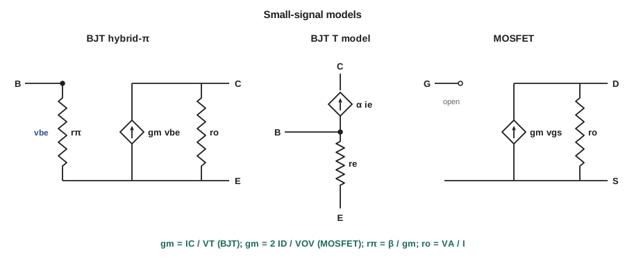
Adding the output resistance r_o = V_A/I_C from the Early effect gives the hybrid-π model: between base and emitter, a resistor r_π; between collector and emitter, a voltage-controlled current source g_m v_be in parallel with r_o. This model is the workhorse of BJT amplifier analysis. At 1 mA with β = 150 and V_A = 100 V: g_m = 40 mS, r_π = 3.75 kΩ and r_o = 100 kΩ. An equivalent T model places a resistance r_e = α/g_m ≈ V_T/I_E, about 25 Ω at 1 mA, in the emitter lead, with the controlled source from collector to base. The T model is often easier to use when there is a resistor in the emitter.
| Parameter | BJT | MOSFET (saturation) |
|---|---|---|
| Transconductance | g_m = I_C / V_T | g_m = 2I_D / v_OV = √(2k_n'(W/L) I_D) |
| Input resistance | r_π = β / g_m | Infinite at DC and low frequency |
| Emitter / source resistance (T model) | r_e = α / g_m ≈ V_T / I_E | 1 / g_m |
| Output resistance | r_o = V_A / I_C | r_o = 1/(λI_D) = V_A / I_D |
| Intrinsic gain g_m r_o | V_A / V_T, often 2,000 to 6,000 | 2V_A / v_OV, often 20 to 200 |
The MOSFET small-signal model
For a MOSFET in saturation, i_D = ½k_n'(W/L)(V_OV + v_gs)². Expanding in the same way gives a linear term and a square term; the linear term defines the MOSFET transconductance,
and the small-signal condition is v_gs much smaller than 2V_OV. The gate draws no current, so the model has an open circuit at the input: a voltage-controlled current source g_m v_gs from drain to source in parallel with r_o. Each of the three forms of g_m is useful. The middle one is the most revealing: at a given current, g_m is set by the overdrive, and a MOSFET at V_OV = 0.2 V has g_m = I_D/0.1 V, while a BJT at the same current has g_m = I_C/0.025 V, four times larger. Equivalently, a MOSFET would need an overdrive of 2V_T ≈ 50 mV to match the BJT, and at such low overdrives the square law is no longer accurate.
Worked problem
Comparing transconductance at 1 mA
Find g_m for a BJT at I_C = 1 mA and for an NMOS at I_D = 1 mA biased with V_OV = 0.5 V, and the intrinsic gain g_m r_o of each, with V_A = 100 V for the BJT and λ = 0.05 V⁻¹ for the MOSFET.
Show solution
- \[g_{m,BJT} = \frac{1\ \text{mA}}{25\ \text{mV}} = 40\ \text{mS}, \qquad r_o = \frac{100}{1\ \text{mA}} = 100\ \text{k}\Omega\]
- \[g_{m,MOS} = \frac{2 \times 1\ \text{mA}}{0.5\ \text{V}} = 4\ \text{mS}, \qquad r_o = \frac{1}{0.05 \times 1\ \text{mA}} = 20\ \text{k}\Omega\]
- \[(g_m r_o)_{BJT} = 4000, \qquad (g_m r_o)_{MOS} = 80\]
Answer: At the same current, the BJT has ten times the transconductance and fifty times the intrinsic gain in this comparison. That is why discrete precision amplifiers often still use bipolar input stages, while the MOSFET's infinite input resistance and easy integration win elsewhere.
Small-signal analysis step by step
Every small-signal problem follows the same recipe. First, solve the DC circuit for the Q-point. Second, compute the small-signal parameters from the bias: g_m, r_π (or r_e) and r_o. Third, draw the small-signal circuit: replace DC supplies by ground, DC current sources by open circuits, coupling and bypass capacitors by short circuits, and the transistor by its model. Fourth, solve that linear circuit for the gain, input resistance and output resistance using nodal analysis or the voltage-divider and parallel-resistance shortcuts from ELE-202. The result is valid only for small signals at mid-band frequencies, where the capacitors are short circuits and the transistor's internal capacitances are still open circuits; lesson 12 deals with the frequencies at which those assumptions fail.
Worked problem
Gain of a simple common-emitter stage
The microphone amplifier's input transistor is biased at I_C = 0.9 mA (β = 150, V_A = 100 V) with R_C = 5.1 kΩ, and its emitter resistor is fully bypassed by a large capacitor. The signal drives the base directly. Find the small-signal voltage gain v_c/v_be.
Show solution
- \[g_m = \frac{0.9\ \text{mA}}{0.025\ \text{V}} = 36\ \text{mS}, \qquad r_o = \frac{100}{0.9\ \text{mA}} \approx 111\ \text{k}\Omega\]
- With the emitter at signal ground, the controlled source g_m v_be drives R_C in parallel with r_o.
- \[A_v = \frac{v_c}{v_{be}} = -g_m (R_C \parallel r_o) = -0.036 \times (5.1\ \text{k} \parallel 111\ \text{k}) \approx -0.036 \times 4.88\ \text{k} \approx -176\]
Answer: The voltage gain is about −176: the output is 176 times larger and inverted. The minus sign means a rising base voltage pulls more current through R_C and lowers the collector voltage.
import math
VT, IC = 0.025, 0.9e-3
gm = IC / VT
RC = 5100.0
# Compare the exact exponential response with the linear small-signal prediction
print(" vbe peak   linear vc    exact +peak   exact -peak   2nd harmonic")
for vbe_pk in (0.001, 0.005, 0.010, 0.020):
    lin = gm * vbe_pk * RC
    up = IC * (math.exp(vbe_pk / VT) - 1) * RC
    dn = IC * (1 - math.exp(-vbe_pk / VT)) * RC
    h2 = vbe_pk / (4 * VT) * 100           # 2nd-harmonic distortion estimate, percent
print(f"{vbe_pk*1000:6.0f} mV {lin:8.3f} V {up:10.3f} V {dn:10.3f} V {h2:5.1f} %") vbe peak linear vc exact +peak exact -peak 2nd harmonic
1 mV 0.184 V 0.187 V 0.180 V 1.0 %
5 mV 0.918 V 1.016 V 0.832 V 5.0 %
10 mV 1.836 V 2.257 V 1.513 V 10.0 %
20 mV 3.672 V 5.625 V 2.528 V 20.0 %The output shows the price of an amplifier with no feedback. With 10 mV at the base, the output's positive peak is about half as large again as its negative peak, which a listener would hear as harsh distortion. Real microphone amplifiers therefore use an unbypassed emitter resistor or overall feedback, trading some gain for linearity, as lesson 11 explains.
Input resistance, output resistance and loading
Gain alone does not describe an amplifier. Any real signal source has its own internal resistance, and any real load draws current, so an amplifier stage is characterized by three numbers: its voltage gain with no load, A_vo; its input resistance R_in, the resistance the source sees looking into the input; and its output resistance R_out, the Thévenin resistance seen looking back into the output with the input signal set to zero. With these three, the stage becomes the simple voltage-amplifier model from ELE-202, and the overall gain from source to load follows from two voltage dividers:
For the common-emitter stage in the last example, R_in is the bias resistors in parallel with r_π, a few kilohms, and R_out is R_C ∥ r_o, about 4.9 kΩ. Amara's electret microphone capsule has an output resistance of about 2 kΩ, comparable to R_in, so roughly a third of the microphone signal is lost at the input before any gain is applied; and if the stage drove a 5 kΩ load directly, half the output would be lost again. Recognizing these divider losses early is what drives the choice of amplifier configuration in lesson 11: a stage with high input resistance at the front, one with low output resistance at the back, and gain in the middle.
Where the models come from in practice
Datasheets for discrete transistors often give small-signal parameters directly as h-parameters, measured at a stated bias: h_fe is the small-signal current gain (close to β), h_ie is the input resistance (close to r_π), and h_oe is the output conductance (1/r_o). Circuit simulators compute all of these automatically from the device model at the DC operating point they find first, exactly the two-step process described here. Hand analysis with simple models is still essential, because it shows which components set the gain and how to change it, which a simulator's numbers alone do not.
Common mistakes
MistakeMixing DC and signal quantities in one circuit.
InsteadSolve DC first, then draw a separate small-signal circuit with DC sources set to zero.
MistakeCalculating g_m from the transistor's part number.
Insteadg_m = I_C/V_T for any BJT; it is set by the bias current.
MistakeUsing the small-signal model for large swings.
InsteadIt is valid only for v_be ≪ 2V_T (or v_gs ≪ 2V_OV); larger signals distort.
MistakeLeaving a power-supply rail as a voltage in the small-signal circuit.
InsteadA DC supply is a short to signals; connect it to signal ground.
Summary and key terms
- Small-signal analysis linearizes a transistor about its Q-point.
- BJT: g_m = I_C/V_T, r_π = β/g_m, r_e ≈ V_T/I_E, r_o = V_A/I_C.
- MOSFET: g_m = 2I_D/V_OV = √(2k_n'(W/L)I_D), infinite gate resistance, r_o = 1/(λI_D).
- At equal current a BJT has more transconductance and intrinsic gain than a MOSFET.
- Recipe: DC analysis, parameters, small-signal circuit with sources zeroed and capacitors shorted, then linear analysis.
- The linear model holds for signals much smaller than 2V_T at a BJT's base–emitter junction.
- Small signal
- A signal small enough that a device's curve is nearly straight over its range.
- Transconductance
- g_m, the change in output current per unit change in input voltage.
- Hybrid-π model
- A BJT model with r_π from base to emitter and g_m v_be in parallel with r_o from collector to emitter.
- T model
- A transistor model with r_e (or 1/g_m) in the emitter or source lead.
- Signal ground
- Any node held at a constant DC voltage, which carries no signal.
- Intrinsic gain
- g_m r_o, the largest voltage gain a single transistor can provide.
- h-parameters
- Small-signal parameters given on datasheets, such as h_fe and h_ie.
Practice problems
Work each problem on paper first, then reveal the answer to check.
Find g_m, r_π and r_e for a BJT at I_C = 2 mA with β = 100.
Show answer
g_m = 80 mS, r_π = 1.25 kΩ, r_e ≈ 12.4 Ω.
An NMOS carries 0.5 mA at V_OV = 0.25 V. Find g_m.
Show answer
2 × 0.5 mA / 0.25 V = 4 mS.
For the NMOS above, what overdrive would give the same g_m as a BJT at 0.5 mA?
Show answer
A BJT has 20 mS; V_OV = 2I_D/g_m = 1 mA / 20 mS = 50 mV.
A stage has g_m = 20 mS and R_C ∥ r_o = 10 kΩ with the emitter at signal ground. Find the gain.
Show answer
−200.
Why is a bypass capacitor treated as a short circuit at mid-band?
Show answer
Its reactance is negligible compared with the resistances around it at signal frequencies.
Find r_o for a BJT at 0.25 mA with V_A = 75 V.
Show answer
300 kΩ.
Lesson quiz · 5 questions
Score 60% or more to complete this lesson.
Create a free account to save your progress, take quizzes and earn a certificate.