Topologies: three-tier, spine-leaf and AI fabrics

A topology is the shape of a network: which switches connect to which, and how many links run between each layer. Technicians do not design topologies, but they cable them, and a technician who understands the shape can look at a row of panels and know what a trunk is for, why there are exactly that many of them, and what will happen if one is unplugged. Nadia spends a morning with Jamal at the whiteboard in the Hall B network row, drawing the three shapes he will meet at Stonebridge: the old three-tier network in parts of Hall A, the spine-leaf fabric in the cloud halls, and the rail-optimized GPU fabric in Hall D.

The three-tier network

Enterprise data centers built before about 2010 usually had three layers of switches. Access switches at the top of each cabinet or the end of each row connected the servers. Aggregation switches, sometimes called distribution switches, connected groups of access switches. A pair of core switches at the top connected the aggregation layer to each other and to the outside world. Traffic from one server to another in a different part of the hall climbed up through the layers and back down, and because only one path could be active at a time, protocols such as spanning tree blocked the spare links to prevent loops.

This shape suited traffic that mostly went in and out of the data center, between users and servers, which network engineers call north-south traffic. It suited modern workloads badly, because applications built from many small services, storage clusters and virtual machines send most of their traffic between servers, east-west, and the three-tier network made that traffic queue at the aggregation switches. Several Hall A customers, Bayview Credit Union among them, still run three-tier networks inside their cages, and Jamal will see their aggregation switches and the blocked spare links on the panels.

Spine-leaf

Most new data center networks are built as a spine-leaf fabric. Every server connects to a leaf switch, usually at the top of its rack or in a network cabinet at the end of its row. Every leaf switch connects to every spine switch. There is no link between two leaves and no link between two spines. Traffic between any two servers on different leaves goes leaf, spine, leaf: always the same number of hops, whichever two servers they are. All the links are active at once, and traffic is spread across the spines by the switches' routing, so losing one spine reduces the fabric's capacity a little rather than cutting anything off.

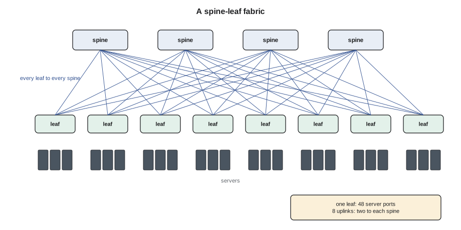
For the cabling, spine-leaf has a very regular shape, which is why it suits structured trunks so well. The number of links between the leaf rows and the spine row is the number of leaves times the number of spines times the links between each pair. The cloud provider in Halls B and C runs exactly this shape, with its leaves at the top of each cabinet and its spines in the hall network rows, and Stonebridge installed the trunks that join them.

Counting a fabric

Nadia shows Jamal how to count a fabric from its design numbers, because the counts tell a technician how many trunks, cassettes and cords to expect on the pallet.

# Spine-leaf: links, oversubscription and the cabling it needs
leaves = 32            # leaf switches, one per cabinet
spines = 8             # spine switches
links_per_pair = 1     # links between each leaf and each spine
server_ports = 48      # server-facing ports per leaf
server_speed = 25      # Gb/s per server port
uplink_speed = 400     # Gb/s per uplink
uplinks = spines * links_per_pair
down = server_ports * server_speed
up = uplinks * uplink_speed
print(f"Uplinks per leaf: {uplinks} x {uplink_speed}G = {up} Gb/s up; {server_ports} x {server_speed}G = {down} Gb/s down")
print(f"Oversubscription {down / up:.2f}:1")
fabric_links = leaves * spines * links_per_pair
print(f"Leaf-to-spine links in the fabric: {fabric_links}")
fibers_per_link = 8            # 400G-DR4 uses 8 of the 12 positions on an MPO
print(f"Strands in use: {fabric_links * fibers_per_link}; MPO trunk legs needed: {fabric_links}")

Uplinks per leaf: 8 x 400G = 3200 Gb/s up; 48 x 25G = 1200 Gb/s down
Oversubscription 0.38:1
Leaf-to-spine links in the fabric: 256
Strands in use: 2048; MPO trunk legs needed: 256

Oversubscription compares the bandwidth a leaf offers its servers with the bandwidth it has toward the spines. A ratio of 1:1 means every server can send at full speed at once; 3:1 means the uplinks could carry only a third of the worst case. Enterprise networks commonly run at 3:1 or so, because servers rarely all send at once. AI training fabrics are built close to 1:1, because the GPUs do all send at once.

Why AI fabrics are different

A training job spreads a model across hundreds or thousands of GPUs. At regular steps, every GPU exchanges results with the others, and the job waits for the slowest exchange to finish. A single slow link holds up every GPU in the job. That has three consequences for the network and its cabling. The fabric must be non-blocking, close to 1:1, at every layer. The links must be very fast, 400 or 800 Gb/s per GPU today, with faster coming. And every link must be clean, because errors that make a link retransmit slow down the whole cluster.

AI clusters actually have several networks. Inside an integrated rack such as the ones Corvid runs in Hall D, the GPUs are joined to each other by a high-speed copper backplane, the scale-up network, which never leaves the rack. Between racks, each GPU has its own network port on a separate backend or scale-out fabric, built as a non-blocking spine-leaf or a variant of it. A frontend network, a more ordinary data center network, connects the servers to storage and to the outside world. And there is a management network, usually 1 Gb/s copper, for the baseboard controllers and the power and cooling equipment. A technician working in Hall D needs to know which of these a cable belongs to, because the backend links are the most sensitive and the most numerous.

Rail-optimized fabrics

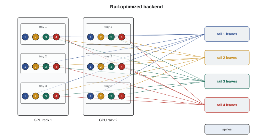
Many AI backend fabrics are built rail-optimized. Each compute tray in Corvid's racks has four GPUs, numbered 1 to 4 in every tray. In a rail-optimized design, GPU 1 of every tray connects to the leaf switches of rail 1, GPU 2 of every tray to rail 2, and so on. Because the training software exchanges data mostly between GPUs with the same number, most traffic stays within one rail and crosses only one leaf. The cabling consequence is that the cables from a rack are not divided by tray but by GPU position: every rack sends a bundle of links to each rail's leaf cabinet, and a cable plugged into the wrong rail works electrically but sends the traffic the long way round, slowing the job.

# A rail-optimized backend fabric for one Hall D pod (illustrative design numbers)
racks = 8
trays_per_rack = 18
gpus_per_tray = 4          # = number of rails
leaf_ports = 64            # 800G ports per leaf switch
down_per_leaf = leaf_ports // 2      # non-blocking: half down, half up
gpus = racks * trays_per_rack * gpus_per_tray
per_rail = gpus // gpus_per_tray
leaves_per_rail = -(-per_rail // down_per_leaf)      # round up
leaves = leaves_per_rail * gpus_per_tray
uplinks = leaves * (leaf_ports - down_per_leaf)
print(f"{gpus} GPUs, {gpus_per_tray} rails of {per_rail} GPUs")
print(f"{leaves_per_rail} leaves per rail, {leaves} leaves, {uplinks} leaf-to-spine links")
print(f"Backend links to cable: {gpus + uplinks}; at 16 strands each that is {(gpus + uplinks) * 16:,} strands")
print(f"Links from each rack to each rail: {trays_per_rack}")

576 GPUs, 4 rails of 144 GPUs
5 leaves per rail, 20 leaves, 640 leaf-to-spine links
Backend links to cable: 1216; at 16 strands each that is 19,456 strands
Links from each rack to each rail: 18

Nearly twenty thousand strands for one pod of eight racks is why Hall D's network rows look so different from Hall A's, and why Stonebridge and Corvid install the backend cabling with pre-terminated trunks rather than individual cords. The numbers are an illustration; Corvid's real design is its own, and Jamal works from its port maps.

Cabling a topology without breaking it

A technician's job in all three shapes is the same: connect the ports the design says, in the order the port map says, and nothing else. But the shape changes what a mistake does. In a three-tier network, a cord moved to the wrong aggregation port can create a loop that spanning tree has to break. In a spine-leaf fabric, a missing uplink reduces capacity and a crossed uplink, a leaf connected to the same spine twice, can confuse the routing. In a rail-optimized fabric, a cable on the wrong rail slows a whole training job. Nadia's rule is that every new fabric link is checked against the port map from both ends, by the label and by the switch's neighbor discovery, before the ticket is closed.

Redundancy in a fabric

Fabrics are built so that no single cable, switch or panel can cut a server off. In a spine-leaf fabric each leaf has links to several spines, so losing one spine or one uplink reduces capacity but leaves every path working. Servers that matter connect to two leaves, one on each side of the cabinet, and the two leaves' uplinks run in separate trunks along separate tray routes where the hall allows. Technicians see this redundancy as rules on the port map: the A-side and B-side trunks of a cabinet never share a tray section, and the two cords of a dual-homed server never go to the same leaf. When Jamal moves a cord, he checks that the move does not leave both of a server's links on the same switch, which would quietly remove its redundancy without any alarm.

AI backend fabrics handle redundancy differently. A training job can usually survive the loss of a link by routing around it or by restarting from its last checkpoint, but it runs more slowly while the link is out. Corvid's operations team would rather have a link fail cleanly than run with errors, which is why its engineers drain a link before any physical work and why a technician never touches a backend cable on a live tray without their word.

Reading the switch's view

Network switches report what they see at each port: whether the link is up, its speed, its error counters and, through neighbor discovery protocols such as LLDP, the name and port of the device at the far end. Technicians at Stonebridge do not configure customer switches, but the customer's engineer can read these values on request, and the cloud provider and Corvid both give Stonebridge read access to the neighbor tables for their fabrics. Comparing the neighbor table with the port map is the fastest way to check that a new link lands where it should, and it is the check that would have caught the rail swap in the example below before anyone noticed a slow job.