Nodal analysis

Series and parallel reduction works only on circuits whose parts happen to line up neatly. A bridge, a network with several sources or a sensor feeding a buffered ADC usually cannot be simplified that way. Nodal analysis is a systematic method that works on any linear circuit. It chooses the node voltages as the unknowns, writes Kirchhoff's current law at each node with the currents expressed through Ohm's law, and solves the resulting set of linear equations. Because it is so systematic, it is also how circuit simulators such as SPICE work internally, and by the end of this lesson you will have written a small simulator of your own.

Jonah's next job on the NS-4 is the temperature sensor. A negative temperature coefficient (NTC) thermistor, whose resistance falls as it warms, sits in a small network with fixed resistors so that the ADC can read temperature over the full roadside range. Ines wants to add a second, fixed reference resistor so firmware can check the ADC's accuracy, and the resulting network is no longer a simple divider.

Node voltages

In nodal analysis one node is chosen as the reference, or ground, and every other node is given a voltage measured relative to it. In a circuit with n nodes there are n − 1 unknown node voltages. Once they are known, every branch voltage is the difference between two node voltages and every resistor current follows from Ohm's law. The choice of reference is free, but choosing the node with the most connections, often the negative terminal of the main supply, usually gives the simplest equations.

The method in its basic form has four steps. First, label the reference node and the remaining node voltages v₁, v₂ and so on. Second, at each non-reference node, write KCL with every current leaving the node expressed as the node's voltage minus the neighboring node's voltage, divided by the resistance between them. Third, collect terms to get one linear equation per node. Fourth, solve the equations by substitution, by matrix methods or by computer.

Writing every current as leaving the node, whatever its real direction, removes the need to guess directions in advance and makes the bookkeeping identical at every node. Current sources are added directly: a source pushing current into the node appears as a known term on the other side of the equation.

Writing the equations

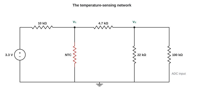
Consider the sensor network in the figure, with the thermistor at 10 kΩ, its value at 25 °C. The 3.3 V source fixes one node directly, so the unknowns are v₁ and v₂. At node 1, three currents leave: back through the 10 kΩ resistor to the 3.3 V node, down through the thermistor, and across the 4.7 kΩ resistor to node 2. At node 2, currents leave back through the 4.7 kΩ resistor, down through the 22 kΩ resistor and down through the 100 kΩ ADC input resistance.

Working in kilohms and milliamperes keeps the numbers tidy; volts divided by kilohms gives milliamperes directly. Collecting terms gives two equations in two unknowns. The pattern of the coefficients is worth noticing: each node's own voltage is multiplied by the sum of the conductances connected to it, and each neighboring node's voltage is multiplied by minus the conductance between them.

The conductance matrix

For a circuit containing only resistors and independent current sources, the node equations always take the form G v = i, where v is the vector of unknown node voltages, i is the vector of source currents injected into each node, and G is the conductance matrix. The matrix can be written by inspection. Each diagonal entry G_jj is the sum of all conductances connected to node j. Each off-diagonal entry G_jk is minus the sum of the conductances connecting nodes j and k. The matrix is therefore symmetric, and for a connected circuit with a reference node it is always invertible.

A voltage source in series with a resistor can be converted into a current source in parallel with the same resistor, a source transformation that lesson 6 justifies. In the sensor network, the 3.3 V source and its 10 kΩ resistor are equivalent to a 0.33 mA source into node 1 in parallel with 10 kΩ to ground, which is why the right-hand side contains 0.33 mA and the diagonal contains the extra 1/10.

Voltage sources and supernodes

A voltage source connected between two non-reference nodes causes a difficulty: its current is unknown and cannot be written with Ohm's law. The solution is the supernode. Draw a boundary around the source and the two nodes it connects, apply KCL to the whole boundary, which avoids the unknown source current, and add the source's constraint equation, the difference between the two node voltages. The count of equations still matches the count of unknowns.

A voltage source connected between a node and the reference is even simpler: it fixes that node's voltage, removing one unknown. This is the usual situation on a digital board, where the supply rails are fixed by regulators and only the signal nodes are unknown.

Dependent sources

Circuits containing amplifiers and transistors are modeled with dependent sources. Nodal analysis handles them by writing the source as if it were independent, then adding an equation that expresses its controlling variable in terms of the node voltages. The resulting G matrix is no longer symmetric, but the method is unchanged. Lesson 7 uses this approach to analyze op-amp circuits with a finite gain.

Solving by computer

Two node equations are easy by hand, but a board with fifty signal nodes is not. Gaussian elimination reduces the system to triangular form by subtracting multiples of one row from the rows below it, then finds the unknowns by back substitution. It costs about n³/3 multiplications for n nodes, so a 50-node circuit needs around 40,000, trivial for a computer. Real simulators exploit the fact that the conductance matrix is sparse, most nodes connecting to only a few others, and solve circuits with millions of nodes. The code below builds the G matrix by stamping each resistor into it, the same idea SPICE uses, and solves the sensor network.

# A tiny nodal-analysis solver: stamp each element into G and i, then solve G v = i
def solve(A, b):
    """Gaussian elimination with partial pivoting."""
    n = len(b)
    M = [row[:] + [b[i]] for i, row in enumerate(A)]
    for col in range(n):
        piv = max(range(col, n), key=lambda r: abs(M[r][col]))
        M[col], M[piv] = M[piv], M[col]
        for r in range(col + 1, n):
            f = M[r][col] / M[col][col]
            for c in range(col, n + 1):
                M[r][c] -= f * M[col][c]
    x = [0.0] * n
    for r in range(n - 1, -1, -1):
        s = M[r][n] - sum(M[r][c] * x[c] for c in range(r + 1, n))
        x[r] = s / M[r][r]
    return x

def nodal(n_nodes, resistors, isources):
    """Nodes are numbered 1..n_nodes; node 0 is ground."""
    G = [[0.0] * n_nodes for _ in range(n_nodes)]
    i = [0.0] * n_nodes
    for a, b, R in resistors:
        g = 1.0 / R
        for p, q in ((a, b), (b, a)):
            if p:
                G[p - 1][p - 1] += g
                if q:
                    G[p - 1][q - 1] -= g
    for node, amps in isources:          # current injected into a node
        i[node - 1] += amps
    return solve(G, i)

def ntc(T_C, R25=10e3, beta=3950.0):   # illustrative thermistor model
    T = T_C + 273.15
    return R25 * 2.718281828 ** (beta * (1 / T - 1 / 298.15))

for T in (-30, 0, 25, 60):
    Rth = ntc(T)
    # the 3.3 V source with 10k becomes 0.33 mA into node 1 with 10k to ground
    v1, v2 = nodal(2, [(1, 0, 10e3), (1, 0, Rth), (1, 2, 4.7e3), (2, 0, 22e3), (2, 0, 100e3)],
                   [(1, 3.3 / 10e3)])
    print("%4d C  Rth = %7.0f ohm  v1 = %.3f V  ADC v2 = %.3f V" % (T, Rth, v1, v2))

 -30 C  Rth =  200204 ohm  v1 = 2.215 V  ADC v2 = 1.757 V
   0 C  Rth =   33621 ohm  v1 = 1.899 V  ADC v2 = 1.507 V
  25 C  Rth =   10000 ohm  v1 = 1.353 V  ADC v2 = 1.073 V
  60 C  Rth =    2486 ohm  v1 = 0.604 V  ADC v2 = 0.479 V

The output shows the ADC voltage rising as the temperature falls, because a colder thermistor has more resistance and takes a larger share of the divider. Across the roadside range from −30 °C to 60 °C the ADC voltage spans about 1.3 V, from 0.48 V to 1.76 V. That is roughly 1,600 steps of a 12-bit converter, about 18 steps per degree on average, which is far finer than the thermistor's own accuracy. Firmware converts the reading back to temperature with a lookup table generated from the same model.

Checking an answer

Nodal analysis produces numbers that are easy to check. Substitute the node voltages back into each KCL equation and confirm the currents balance. Check that the power delivered by the sources equals the power absorbed by the resistors. Check limiting cases: if the thermistor's resistance went to zero, node 1 would be shorted to ground and both node voltages should go to zero; if it went to infinity, the network would become a simple chain of resistors that you can solve with the divider rule. A solver that passes these tests is very likely correct.