
CHE-314 · Lesson 7 of 12 · 23 min
Interphase mass transfer and overall coefficients
With diffusivities and coefficients in hand, Theo turns to the heart of the scrubber: ethanol leaves the gas, crosses the gas-liquid interface and enters the water. He has a coefficient for each side, but neither the interface compositions nor the area of the wetted packing can be measured directly. Ingrid sketches the problem on the whiteboard the way Lewis and Whitman did a century ago: two films, one on each side of the interface, in series. The idea leads to overall coefficients, which can be used with bulk compositions alone, and it tells a designer which side of the interface controls the rate. That answer changes completely from one solute to another.
Phase equilibrium at the interface
Transfer between phases is driven by their departure from equilibrium, so the equilibrium relationship comes first. For a dilute solute in a liquid in contact with a gas, the mole fraction in the gas at equilibrium is usually proportional to the mole fraction in the liquid over a useful range:
The slope \(m\) is dimensionless. For gases that are sparingly soluble, such as oxygen and carbon dioxide in water, it comes from Henry's law in the form \(p_A = H x_A\), so \(m = H/P\), where \(H\) is the Henry's law constant in pressure units and \(P\) is the total pressure. For a volatile organic solute such as ethanol, the equilibrium comes from the modified Raoult's law of CHE-250 and CHE-220: \(y_A P = \gamma_A x_A P_A^{\mathrm{sat}}\), so for dilute solutions \(m = \gamma_A^\infty P_A^{\mathrm{sat}}/P\), where \(\gamma_A^\infty\) is the activity coefficient at infinite dilution. Henry's law constants are reported in at least a dozen different unit systems, some inverted, so Theo always converts to \(m\) before using one.
| Solute in water, 32 °C | Source of m | Approximate m |
|---|---|---|
| oxygen | Henry constant about 4.9 × 10⁴ bar | 48,000 |
| carbon dioxide | Henry constant about 1,900 bar | 1,900 |
| acetaldehyde | Henry data | about 5 |
| ammonia | Henry data | about 0.8 |
| ethanol | γ∞ ≈ 5, vapor pressure 11.6 kPa | about 0.57 |
The table shows the enormous range of \(m\). Oxygen has a slope of tens of thousands: at equilibrium the liquid holds very little of it. Ethanol has a slope below 1: water holds ethanol readily. All slopes rise with temperature, because solubility falls, which is why scrubbers prefer cool water.
The two-film model
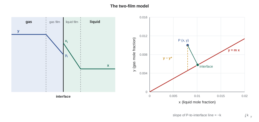
The two-film model places a gas film and a liquid film on either side of the interface. Each film carries the flux by its own coefficient, and the interface itself offers no resistance, so the two phases are in equilibrium right at the interface. At steady state, with no accumulation at the interface, the same flux crosses both films:
Here \(y_A\) and \(x_A\) are bulk mole fractions and \(y_{Ai}\) and \(x_{Ai}\) are interface values. The equations can be solved for the interface compositions: \(x_{Ai} = (k_y y_A + k_x x_A)/(k_y m + k_x)\). Graphically, on a plot of \(y\) against \(x\), the point representing the bulk phases lies off the equilibrium line, and a straight line from that point with slope \(-k_x/k_y\) meets the equilibrium line at the interface composition.
Overall coefficients
The interface compositions are rarely known, so it is more convenient to write the flux with a driving force made from bulk compositions alone. Define \(y_A^* = m x_A\), the gas mole fraction that would be in equilibrium with the bulk liquid. The overall gas-phase coefficient \(K_y\) is defined by \(N_A = K_y(y_A - y_A^*)\). Adding the film resistances, using \(y_{Ai} - y_A^* = m(x_{Ai} - x_A)\), gives
This is the mass transfer version of adding thermal resistances in series, with one important difference: the liquid resistance is multiplied by the equilibrium slope \(m\). A large \(m\) makes the liquid resistance dominate; a small \(m\) makes the gas resistance dominate. The same relationships hold for volumetric coefficients, \(1/K_ya = 1/k_ya + m/k_xa\), which is how packed columns are designed. The relation assumes a straight equilibrium line over the range between the interface and bulk compositions; for curved lines, the local slope must be used.
Which side controls?
For the scrubber packing, Theo uses film coefficients typical of 50 mm metal rings at the expected flows: \(k_ya \approx 150\) and \(k_xa \approx 300\) mol/(m\(^3\) s). He then computes the share of the total resistance on each side for several solutes.
# Interphase mass transfer: equilibrium, the two-film model and overall coefficients
import math
P_bar = 1.013
# Equilibrium slopes m in y = m x at 32 C (approximate)
H_CO2 = 1900.0                     # bar, Henry constant x = p/H
H_O2 = 4.9e4                       # bar
gamma_inf, p_sat_e = 5.0, 11.6     # ethanol in water: infinite-dilution activity coefficient, vapor pressure kPa
m = {'CO2': H_CO2 / P_bar, 'O2': H_O2 / P_bar, 'ethanol': gamma_inf * p_sat_e / 101.3, 'ammonia': 0.8}
for k, v in m.items():
    print(f"m({k}) = {v:.3g}")

kya, kxa = 150.0, 300.0           # mol/(m3 s), volumetric film coefficients in the packed scrubber
print("solute     1/Kya (s m3/mol)   gas-film share   liquid-film share")
for k, mv in m.items():
    rg, rl = 1 / kya, mv / kxa
    Kya = 1 / (rg + rl)
    print(f"{k:9s}  {1 / Kya:.3e}          {rg / (rg + rl) * 100:6.1f} %        {rl / (rg + rl) * 100:6.1f} %")

# Interface compositions at one point in the scrubber for ethanol
y, x = 0.010, 0.0080               # bulk gas and liquid mole fractions at this height
mv = m['ethanol']
# ky (y - yi) = kx (xi - x) with yi = m xi  ->  xi = (ky y + kx x) / (ky m + kx)
xi = (kya * y + kxa * x) / (kya * mv + kxa)
yi = mv * xi
y_star = mv * x
Kya = 1 / (1 / kya + mv / kxa)
print(f"interface: yi = {yi:.5f}, xi = {xi:.5f}; y* = m x = {y_star:.5f}")
print(f"rate per volume: ky a (y - yi) = {kya * (y - yi):.3f}, Ky a (y - y*) = {Kya * (y - y_star):.3f} mol/(m3 s)")m(CO2) = 1.88e+03 m(O2) = 4.84e+04 m(ethanol) = 0.573 m(ammonia) = 0.8 solute 1/Kya (s m3/mol) gas-film share liquid-film share CO2 6.259e+00 0.1 % 99.9 % O2 1.612e+02 0.0 % 100.0 % ethanol 8.575e-03 77.7 % 22.3 % ammonia 9.333e-03 71.4 % 28.6 % interface: yi = 0.00579, xi = 0.01011; y* = m x = 0.00458 rate per volume: ky a (y - yi) = 0.632, Ky a (y - y*) = 0.632 mol/(m3 s)
The result is striking. For oxygen and carbon dioxide, essentially all the resistance is in the liquid film: these are liquid-film-controlled systems, and improving the gas-side flow does nothing. That is why fermenters are designed for large \(k_La\) values and why the gas-side coefficient never appears in lesson 5. For ethanol, about 78 % of the resistance is in the gas film, and for ammonia about 71 %: these solutes are mostly gas-film controlled. Improving the liquid side helps them only a little, while anything that thins the gas film, such as higher gas velocity or packing with more area, helps a lot. Acetaldehyde, with \(m\) about 5, sits in between, with most of its resistance on the liquid side, a fact that matters in lesson 12.
Worked problem
Interface compositions in the scrubber
At one height in the scrubber, the bulk gas holds \(y = 0.010\) ethanol and the bulk liquid \(x = 0.0080\). With \(m = 0.57\), \(k_ya = 150\) and \(k_xa = 300\) mol/(m\(^3\) s), find the interface compositions and the rate of transfer per unit volume.
Show solution
- \(x_i = (150 \times 0.010 + 300 \times 0.0080)/(150 \times 0.57 + 300) = 3.90/385.5 = 0.0101\); \(y_i = 0.57 \times 0.0101 = 0.00579\).
- Gas side: \(k_ya(y - y_i) = 150 \times (0.010 - 0.00579) = 0.632\) mol/(m\(^3\) s).
- Overall: \(K_ya = 1/(1/150 + 0.57/300) = 116.6\); \(y^* = 0.57 \times 0.0080 = 0.00456\); \(K_ya(y - y^*) = 0.632\) mol/(m\(^3\) s).
Answer: The film and overall calculations agree, as they must. Most of the driving force, from 0.010 down to 0.0058, is spent crossing the gas film.
Telling the resistances apart in practice
Film coefficients are rarely measured one at a time in plant equipment, but engineers can still find out which side controls. One way is to absorb a solute whose resistance is known to lie almost entirely on one side. Absorbing oxygen or carbon dioxide into water, or desorbing them, measures \(k_xa\) alone, because their huge \(m\) makes the gas film irrelevant. Absorbing ammonia into dilute acid, where the reaction keeps the liquid-side resistance near zero, measures \(k_ya\) alone. Packing vendors use exactly these test systems to publish \(H_L\) and \(H_G\) data for their products. A second way is to vary one flow at a time: if raising the gas rate raises the overall coefficient roughly as the gas-side correlation predicts and raising the liquid rate does little, the gas side controls. Theo plans such a test on the new scrubber after start-up, so that later changes, such as warmer water or a different packing, can be predicted from plant data rather than from textbook correlations.
Worked problem
Carbon dioxide dissolving into the scrubber water
Some carbon dioxide from the vent gas also dissolves into the scrubber water. With \(m = 1900\), \(k_ya = 150\) and \(k_xa = 300\) mol/(m\(^3\) s), what is \(K_ya\), and what does it say about how much carbon dioxide the water picks up?
Show solution
- \(1/K_ya = 1/150 + 1900/300 = 0.0067 + 6.33 = 6.34\) s m\(^3\)/mol, so \(K_ya = 0.158\) mol/(m\(^3\) s).
- The gas is almost pure carbon dioxide, so \(y \approx 0.985\), while water in equilibrium with it holds only \(x = y/m \approx 5\times10^{-4}\).
- The water leaving can approach saturation at about \(5\times10^{-4}\) mole fraction, roughly 1.2 g of carbon dioxide per liter.
Answer: The water leaves nearly saturated with carbon dioxide, which makes it mildly acidic. That is harmless in the slurry tank but matters for the choice of pipe and pump materials, as CHE-280 explained.
Concentrated solutions and curved equilibrium
The simple sum of resistances works for dilute solutions with straight equilibrium lines. When the equilibrium line curves, as it does for ethanol in water above a few mole percent, \(m\) in the overall coefficient must be the slope of the chord between the interface and equilibrium points, which changes along the column. In concentrated gases, the film coefficients themselves also change with composition through the bulk-flow factor. Designers then either work with film coefficients and interface compositions, solving for the interface at each point, or divide the column into sections with nearly constant slopes. For the vent scrubber, with ethanol below 2 mol % in both phases, the dilute approach is accurate.
Temperature and heat effects
Absorption releases heat: dissolving ethanol into water gives off roughly its heat of condensation plus a small heat of mixing. In a dilute scrubber the heat raises the water temperature by only a degree or two, and the column can be treated as isothermal at the water temperature. In concentrated absorbers, such as ammonia into water or carbon dioxide into amine solutions, the temperature rise can be tens of degrees and shift the equilibrium enough to need a heat balance alongside the mass balance, a point CHE-350 develops. Theo notes for the design file that summer water at 32 °C, rather than the 20 °C of winter, nearly doubles \(m\) for ethanol, mainly through the vapor pressure, which is the condition the scrubber must be sized for.
Common mistakes
MistakeUsing a Henry's law constant without checking its units and definition.
InsteadConvert it to \(m = y^*/x\) at the operating pressure before use.
MistakeAdding film resistances without the equilibrium slope.
Instead\(1/K_y = 1/k_y + m/k_x\); the liquid term carries \(m\).
MistakeImproving gas mixing to speed up oxygen transfer.
InsteadOxygen transfer is liquid-film controlled; improve \(k_La\) instead.
MistakeUsing one value of \(m\) where the equilibrium line curves.
InsteadUse the local chord slope or work with film coefficients section by section.
Summary and key terms
- For dilute solutions, the equilibrium relationship is often linear: \(y^* = mx\).
- Henry's law gives \(m = H/P\) for sparingly soluble gases; modified Raoult's law gives \(m = \gamma^\infty P^{\mathrm{sat}}/P\) for volatile solutes.
- The two-film model places equilibrium at the interface and a resistance in each phase.
- Overall coefficients use bulk compositions: \(1/K_y = 1/k_y + m/k_x\).
- Large \(m\) (oxygen, carbon dioxide) means liquid-film control; small \(m\) (ethanol, ammonia) means mostly gas-film control.
- Higher temperature raises \(m\) and makes absorption harder.
- Henry's law
- A linear relationship between the partial pressure of a dilute solute and its liquid mole fraction.
- Equilibrium slope
- The ratio m = y*/x for dilute solutions.
- Two-film model
- A model with a gas film and a liquid film in series and equilibrium at the interface.
- Overall coefficient
- A coefficient defined with a driving force from bulk compositions, combining both film resistances.
- Gas-film control
- A condition in which most of the resistance to transfer lies in the gas phase.
- Liquid-film control
- A condition in which most of the resistance lies in the liquid phase.
- Interface composition
- The equilibrium pair of gas and liquid compositions at the phase boundary.
Practice problems
Work each problem on paper first, then reveal the answer to check.
A Henry's law constant is 3,000 bar. What is \(m\) at 2 bar total pressure?
Show answer
\(m = 3000/2 = 1500\).
With \(k_ya = 100\), \(k_xa = 200\) mol/(m\(^3\) s) and \(m = 2\), what share of the resistance is in the gas film?
Show answer
\(0.01/(0.01 + 0.01) = 50\%\).
Why does improving gas-side turbulence not help oxygen transfer to a fermenter?
Show answer
The liquid film holds nearly all the resistance.
What line on a \(y\)–\(x\) diagram connects the bulk point to the interface point?
Show answer
A straight line with slope \(-k_x/k_y\).
Write \(1/K_x\) in terms of the film coefficients.
Show answer
\(1/K_x = 1/(mk_y) + 1/k_x\).
Why are scrubbers sized for summer water temperatures?
Show answer
Warmer water raises \(m\), reducing the absorption driving force.
Lesson quiz · 5 questions
Score 60% or more to complete this lesson.
Create a free account to save your progress, take quizzes and earn a certificate.