Mass transfer correlations and the heat-mass transfer analogy

Wren Halvorsen is updating the plant's emergency response plan, and she has a question that needs a number: if an ethanol transfer hose fails at the loadout and leaves a pool on the concrete, how fast does the ethanol evaporate? The answer sets how quickly vapor builds up near the pool and how much time responders have to contain it with foam. Theo realizes the question is the same as the ones in heat transfer textbooks about air blowing over a warm plate, with mass in place of heat. This lesson collects the standard correlations for mass transfer coefficients and shows how the analogy with heat transfer lets engineers borrow results from one field for the other.

Dimensionless groups for mass transfer

Mass transfer coefficients are correlated with the same strategy as heat transfer coefficients: express the coefficient as a dimensionless number and relate it to dimensionless groups that describe the flow and the fluid. The Sherwood number is the dimensionless coefficient; the Schmidt number is the ratio of momentum diffusivity to mass diffusivity, a property of the fluid and solute:

The Sherwood number matches the Nusselt number \(hL/k\), and the Schmidt number matches the Prandtl number \(\nu/\alpha\). For gases, \(Sc\) is between about 0.2 and 3: for ethanol in air at 25 °C it is \(1.56\times10^{-5}/1.25\times10^{-5} = 1.25\). For dissolved solutes in water it is about 500 to 1,000, because liquid diffusivities are so small. That huge Schmidt number means the concentration boundary layer in a liquid is far thinner than the velocity boundary layer, the mass transfer counterpart of the very thin thermal layer in oils.

Flow over a flat surface

For flow along a flat surface of length \(L\), boundary-layer theory gives the average Sherwood number in laminar flow, and an empirical form covers turbulent flow:

These are the same as the flat-plate heat transfer correlations with \(Nu\) replaced by \(Sh\) and \(Pr\) by \(Sc\). They hold for low mass transfer rates, where the flow of material across the surface does not disturb the boundary layer. Evaporation of a volatile liquid such as ethanol at room temperature satisfies that condition reasonably well; very high rates, such as a liquid near its boiling point, need a blowing correction.

Spheres, cylinders and droplets

For a single sphere, the Ranz-Marshall correlation adds a convective term to the pure-diffusion limit \(Sh = 2\) from lesson 3:

It applies to droplets evaporating in a spray, particles dissolving in a stirred liquid and grains drying in a hot gas stream, with \(Re\) based on the relative velocity between particle and fluid. For small droplets moving slowly, the 2 dominates, so \(k_c \approx 2D_{AB}/d\) and small droplets have very large coefficients: a 200 µm droplet in air has \(k_c\) of about 0.2 m/s. Similar correlations exist for cylinders in cross flow, used for wetted wires and for the tubes of evaporative coolers.

Flow inside pipes and wetted-wall columns

For turbulent flow inside a tube whose wall dissolves or is wetted by a liquid film, the classic correlation of Linton and Sherwood, and the wetted-wall data of Gilliland and Sherwood, follow the Dittus-Boelter form of heat transfer:

Wetted-wall columns, in which liquid runs down the inside of a vertical tube while gas flows up the core, were the original tool for measuring gas-side coefficients and diffusivities, because their interfacial area is known exactly. They remain useful in research laboratories, but packed columns and structured packings, whose correlations lesson 9 introduces, dominate industrial practice.

The Chilton-Colburn analogy

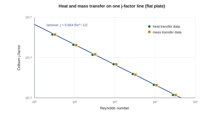
Comparing the heat and mass transfer correlations, Chilton and Colburn noticed in the 1930s that both could be written with the same function of Reynolds number by defining two \(j\)-factors:

The equality \(j_H = j_D\) holds well for flow over flat plates, around cylinders and spheres and in pipes, in the range \(0.6 < Sc < 3000\), as long as there is no form drag effect in the comparison with friction. The comparison with the friction factor \(f\) applies only where skin friction is the whole of the drag, such as flat plates and pipes, not bluff bodies. In practice the analogy lets an engineer who has a measured or correlated heat transfer coefficient for some geometry obtain the mass transfer coefficient for the same geometry and flow:

This is the basis of the wet-bulb thermometer and of cooling tower design in lesson 10, where heat and mass transfer happen together at the same air-water interface. It also lets designers use the large body of heat transfer data for odd geometries, such as finned surfaces, when mass transfer data are missing.

Packed beds and other geometries

For a fluid flowing through a bed of particles, such as gas through adsorbent beads or liquid through a catalyst bed, the particles disturb the flow strongly and the coefficients are higher than for a single sphere at the same velocity. A correlation by Wakao and Funazkri, \(Sh = 2 + 1.1\,Re^{0.6}Sc^{1/3}\), with \(Re\) based on the particle diameter and the superficial velocity, is widely used for gases and liquids. Handbooks list dozens of others, for stirred tanks, bubble columns, rotating discs and membranes, each with its own range of validity. Theo's rule is to use the correlation that was developed for the geometry and flow at hand, check that the dimensionless groups fall inside its tested range, and expect a scatter of 20 to 30 % even then.

Stirred tanks and bubble columns

Gas-liquid contactors with bubbles, such as the propagation tank of lesson 5 and the much larger fermenters, have their own correlations. Because the bubble area and the coefficient are hard to separate, they are usually written for \(k_La\) directly, in the form \(k_La = C\,(P_g/V)^{\alpha}\,u_s^{\beta}\), where \(P_g/V\) is the gassed power input per unit volume, \(u_s\) is the superficial gas velocity, and the constants depend on the liquid. For water and thin broths, exponents near 0.4 to 0.7 for power and 0.2 to 0.6 for gas velocity are typical. Salts, sugars and surfactants change bubble coalescence and can shift \(k_La\) by a factor of two or more, so correlations measured in clean water are only a starting point for real fermentation broths. In bubble columns, where there is no agitator, \(k_La\) depends mainly on the superficial gas velocity, and values of 0.01 to 0.1 s\(^{-1}\) are common. These correlations explain why the propagation tanks run their agitators hard and why the sparger matters so much: halving the bubble size roughly doubles the interfacial area for the same air flow.

# Mass transfer correlations and the heat-mass transfer analogy
import math
R, T, P = 8.314, 298.15, 101325.0
c = P / (R * T)
nu_air = 1.56e-5            # m2/s, kinematic viscosity of air at 25 C
D_e = 1.25e-5               # m2/s, ethanol in air (lesson 2)
Sc = nu_air / D_e
print(f"Schmidt number, ethanol in air = {Sc:.2f}")

# 1. Evaporation from an ethanol spill pool (flat plate, wind along the pool)
u, Lp, W = 3.0, 2.0, 2.0    # m/s wind, m pool length, m pool width
Re = u * Lp / nu_air
if Re < 5e5:
    Sh = 0.664 * Re ** 0.5 * Sc ** (1 / 3)
else:
    Sh = 0.037 * Re ** 0.8 * Sc ** (1 / 3)
kc = Sh * D_e / Lp
p_sat = 7.87e3               # Pa at 25 C
yA = p_sat / P
N = kc * c * math.log(1 / (1 - yA))     # mol/(m2 s), diffusion through stagnant air
m_dot = N * Lp * W * 0.04607 * 3600     # kg/h
print(f"Re_L = {Re:.3g}, Sh = {Sh:.0f}, k_c = {kc * 1000:.2f} mm/s")
print(f"evaporation from the 4 m2 pool = {m_dot:.1f} kg/h")

# 2. A falling droplet or particle: Ranz-Marshall, Sh = 2 + 0.6 Re^0.5 Sc^(1/3)
d, v = 200e-6, 0.5           # m, m/s relative velocity
Re_p = v * d / nu_air
Sh_p = 2 + 0.6 * Re_p ** 0.5 * Sc ** (1 / 3)
print(f"droplet: Re = {Re_p:.2f}, Sh = {Sh_p:.2f}, k_c = {Sh_p * D_e / d:.3f} m/s")

# 3. Turbulent flow in a tube, wetted-wall or dissolving wall: Sh = 0.023 Re^0.83 Sc^0.33
d_t, v_t = 0.025, 5.0
Re_t = v_t * d_t / nu_air
Sh_t = 0.023 * Re_t ** 0.83 * Sc ** 0.33
print(f"tube: Re = {Re_t:.0f}, Sh = {Sh_t:.1f}, k_c = {Sh_t * D_e / d_t * 1000:.1f} mm/s")

# 4. Chilton-Colburn analogy: get k_c from a measured heat transfer coefficient
h, rho, cp, Pr = 35.0, 1.18, 1007.0, 0.71   # W/(m2 K) over the same surface, air properties
kc_analogy = h / (rho * cp) * (Pr / Sc) ** (2 / 3)
print(f"analogy: h = {h} W/(m2 K) gives k_c = {kc_analogy * 1000:.1f} mm/s")

# 5. Packed bed of adsorbent beads (Wakao-Funazkri), Sh = 2 + 1.1 Re^0.6 Sc^(1/3)
dp, us, nu_v, D_v = 3.0e-3, 0.30, 1.6e-5, 1.4e-5    # bead diameter, superficial velocity, properties of the hot gas
Re_b = us * dp / nu_v
Sh_b = 2 + 1.1 * Re_b ** 0.6 * (nu_v / D_v) ** (1 / 3)
print(f"packed bed: Re = {Re_b:.1f}, Sh = {Sh_b:.2f}, k_c = {Sh_b * D_v / dp * 1000:.1f} mm/s")

Schmidt number, ethanol in air = 1.25
Re_L = 3.85e+05, Sh = 443, k_c = 2.77 mm/s
evaporation from the 4 m2 pool = 6.1 kg/h
droplet: Re = 6.41, Sh = 3.64, k_c = 0.227 m/s
tube: Re = 8013, Sh = 43.0, k_c = 21.5 mm/s
analogy: h = 35.0 W/(m2 K) gives k_c = 20.2 mm/s
packed bed: Re = 56.2, Sh = 14.91, k_c = 69.6 mm/s

The output puts the coefficients side by side: under 3 mm/s for the spill pool, about 20 mm/s for the tube and the finned surface, about 70 mm/s for small beads in a packed bed and over 200 mm/s for a small droplet. Coefficients get larger as the characteristic length shrinks, because the boundary layers get thinner. That is the logic behind random and structured packings, sprays and small adsorbent beads: create a large area and thin boundary layers at the same time.