
BUS-230 · Lesson 5 of 12 · 32 min
Facility location and layout
Where an operation is located and how its space is arranged shape its costs, its service and its ability to grow for years. A distribution center placed a few hours closer to its main markets can save millions in transport costs and offer next-day delivery; a clinic placed on a bus route serves patients who do not drive; a factory layout that forces materials to criss-cross the floor wastes labor, damages parts and hides problems. Location and layout decisions are expensive to reverse, so they deserve careful analysis even though many of the factors involved are hard to quantify.
This lesson covers the factors that drive location decisions, three quantitative methods (factor rating, locational cost–volume analysis and the center-of-gravity method), location decisions for services, the main types of layout, and assembly-line balancing. The crossover analysis from lesson 2 and the bottleneck concept from lesson 3 reappear here.
Location decisions and their drivers
Location decisions are usually made in stages: first the country or region, then the community, then the specific site. At the country level, firms weigh labor costs and productivity, market access, trade agreements and tariffs, exchange rates, political stability, regulation, taxes, infrastructure and culture. At the community level, they weigh the availability of skilled workers, wage rates, utilities, transport links, quality of life for employees, local attitudes and incentives. At the site level, they weigh land cost, size and zoning, access to highways, rail, ports or airports, environmental conditions, and room for future expansion.
Different operations weigh these factors differently. Manufacturers of heavy, low-value products such as cement or beverages locate close to markets because transport costs are high relative to value; processors of perishable or bulky raw materials, such as fish plants, pulp mills and mines, locate close to their inputs. Firms that depend on scarce skills locate in talent clusters: software in Toronto–Waterloo, Montréal, Vancouver, Seattle or Austin; aerospace in Montréal and Wichita; automotive along the Ontario–Michigan–Ohio corridor. Clusters offer specialized suppliers, shared knowledge and deep labor pools, which is why they persist even where costs are high.
Global location strategies have shifted in recent years. After decades of offshoring production to low-cost countries, many firms are reconsidering. Rising wages abroad, long and fragile supply chains exposed by the pandemic, shipping disruptions, tariffs and trade tensions, and concerns about forced labor and emissions have encouraged reshoring (bringing production home), nearshoring (moving it to nearby countries such as Mexico) and friend-shoring (moving it to politically allied countries). Lesson 12 discusses the supply chain risks behind these moves. The right answer depends on total landed cost and risk, not labor cost alone.
| Program type | US examples | What to check |
|---|---|---|
| State and local incentives | Tax abatements, grants, infrastructure and training funds offered by states and cities | Job and investment commitments and clawback clauses |
| Federal tax and grant programs | Manufacturing and clean-energy credits, semiconductor grants and Opportunity Zones | Current status, which changes with legislation |
| Customs programs | Foreign-trade zones, which defer or reduce duties on imported inputs | Whether goods are re-exported or enter US commerce |
| Workforce programs | State workforce training grants and community college partnerships | Training obligations and reporting |
Factor rating
The factor-rating method introduced in lesson 2 is the most widely used location tool because it can combine quantitative and qualitative factors. The team lists relevant factors, assigns weights that sum to 1, scores each candidate location on each factor (for example from 1 to 100), multiplies scores by weights and sums them. Its value lies as much in the discussion it forces as in the final number. Sensitivity analysis is essential: if a small change in a weight reverses the ranking, the decision is a close call and deserves more investigation.
Worked problem
Rating two sites for a call center
A firm compares two cities for a 300-seat customer contact center. Weights: labor availability 0.30, wage cost 0.25, telecom and power reliability 0.20, office cost 0.15, quality of life 0.10. City X scores 80, 60, 90, 70 and 85; City Y scores 65, 85, 75, 90 and 70. Which city ranks higher?
Show solution
- City X: 0.30 × 80 + 0.25 × 60 + 0.20 × 90 + 0.15 × 70 + 0.10 × 85 = 24 + 15 + 18 + 10.5 + 8.5 = 76.0.
- City Y: 0.30 × 65 + 0.25 × 85 + 0.20 × 75 + 0.15 × 90 + 0.10 × 70 = 19.5 + 21.25 + 15 + 13.5 + 7 = 76.25.
- The scores differ by only 0.25 points, well within the uncertainty of the scoring.
- If labor availability is weighted 0.35 and wage cost 0.20, X scores 77.0 and Y 75.25, reversing the ranking.
Answer: The cities are effectively tied; the decision depends on how much weight the firm places on labor availability versus wage cost, so management should investigate both factors more closely before choosing.
Locational cost–volume analysis
When the main differences between sites are in fixed and variable costs, the crossover method from lesson 2 applies directly. Fixed costs include rent or construction, property taxes and overheads; variable costs include labor, materials and transport per unit. Plotting total cost against volume for each site shows which is cheapest at each volume. For example, if site A has fixed costs of $300,000 a year and variable costs of $75 a unit, site B $600,000 and $45, and site C $1,100,000 and $25, then A is cheapest below 10,000 units, B between 10,000 and 25,000 units, and C above 25,000 units. At an expected volume of 20,000 units, B is the low-cost choice.
The center-of-gravity method
When transport cost is the main concern, the center-of-gravity method finds a location that minimizes the volume-weighted distance to the points it serves, such as the stores a distribution center supplies. Each destination is placed on a coordinate grid (a map with x and y coordinates) and weighted by the volume shipped to it. The center of gravity is the weighted average of the coordinates:
where \(d_{ix}\) and \(d_{iy}\) are the coordinates of destination \(i\) and \(V_i\) is the volume shipped there. The result is a starting point rather than a final answer: it uses straight-line distance, ignores the road network, and may land on a lake, a residential area or an expensive site. Analysts then examine nearby real sites with road and highway access, often using geographic information systems (GIS) and network optimization software that model actual travel times and costs.
Worked problem
Locating a regional distribution center
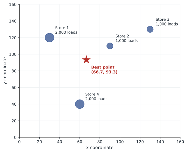
A retailer ships to four stores. On a grid map, store 1 is at (30, 120) and receives 2,000 loads a year; store 2 at (90, 110), 1,000 loads; store 3 at (130, 130), 1,000 loads; store 4 at (60, 40), 2,000 loads. Find the center of gravity.
Show solution
- Total volume = 2,000 + 1,000 + 1,000 + 2,000 = 6,000 loads.
- Cx = (30 × 2,000 + 90 × 1,000 + 130 × 1,000 + 60 × 2,000) ÷ 6,000 = 400,000 ÷ 6,000 ≈ 66.7.
- Cy = (120 × 2,000 + 110 × 1,000 + 130 × 1,000 + 40 × 2,000) ÷ 6,000 = 560,000 ÷ 6,000 ≈ 93.3.
- The retailer should look for sites near (67, 93) with good highway access, then compare actual road distances and costs.
Answer: The center of gravity is at about (66.7, 93.3), pulled toward the two high-volume stores. It is a starting point for evaluating real sites.
Locating services
For services, location is primarily about revenue rather than cost, because customers must travel to the service or the service must travel to them. Retailers, restaurants, banks and clinics study the demographics, incomes and purchasing power of the surrounding area, traffic counts, visibility, parking, transit access and the presence of competitors and complementary businesses. Gravity models of retail, such as the Huff model, estimate the probability that a customer will shop at a store based on its size or attractiveness and the customer's travel time to it and to competing stores.
Public services face different goals. A fire station or ambulance base is located to keep response times below a target for as much of the population as possible; a library or community center to maximize access, often with attention to equity for underserved neighborhoods. Online services have changed the picture: many retailers now locate stores partly as showrooms and pickup points and locate fulfillment centers to cover the largest population within a one- or two-day delivery radius.
Types of layout
Layout is the physical arrangement of departments, workstations, equipment and storage within a facility. A good layout minimizes material and people movement, uses space efficiently, makes the flow of work visible, supports safety and communication, and is flexible enough to adapt as products and volumes change. The main types follow the process types from lesson 3.
| Layout type | Arrangement | Best for | Example |
|---|---|---|---|
| Process (functional) | Similar equipment or activities grouped together | Low volume, high variety; job shops | Hospital departments; machine shop with lathe, milling and drilling areas |
| Product (line) | Stations arranged in the sequence of operations | High volume, standardized products | Appliance assembly line; cafeteria line |
| Cellular | Machines grouped into cells, each making a family of similar parts | Moderate volume and variety | Cell making a family of valve bodies |
| Fixed-position | Product stays put; workers, materials and equipment come to it | Large, bulky projects | Shipbuilding, construction, aircraft assembly |
| Retail and service | Arranged to expose customers to products and guide flow | Stores, restaurants, banks | Grocery store with staples at the back |
| Warehouse | Storage arranged to balance space and picking travel | Distribution centers | Fast movers placed nearest the shipping dock |
In a process layout, the main design problem is to place departments so that those with heavy traffic between them are close together. A load–distance score multiplies the number of loads moved between each pair of departments by the distance between them and sums the products; alternative layouts are compared by their scores, and analysts swap department locations to reduce the total. Hospitals, for example, place emergency departments next to imaging and close to operating rooms. Cellular layouts, a feature of lean operations (lesson 11), regroup a process layout into cells, often U-shaped, that make families of similar parts; they cut travel, waiting and work in process and let a small team own a product from start to finish.
Office and service layouts increasingly balance collaboration and focus. Open-plan offices encourage interaction but can reduce concentration; many organizations now use a mix of open areas, quiet rooms and bookable spaces, especially with hybrid work. Warehouse layouts use the principle of placing the fastest-moving items closest to the dock, a version of ABC analysis (lesson 9), and many now include automated storage and robotic picking, discussed in ROB-440.
Line balancing
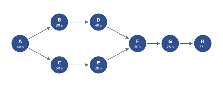
In a product layout, the central problem is assembly-line balancing: assigning tasks to workstations so that each station's work fits within the required cycle time and idle time is minimized, while respecting precedence (some tasks must come before others). The required cycle time is set by demand and is called takt time, from the German word for the beat of music:
The theoretical minimum number of stations is the total work content divided by the takt time, rounded up. Because tasks cannot be split and precedence must be respected, the actual number is often higher. Heuristic rules assign tasks one station at a time: among tasks whose predecessors are complete and that fit in the time remaining at the station, choose the one with the longest task time (or the most followers). Efficiency is the total work content divided by the number of stations multiplied by the cycle time; balance delay is one minus efficiency.
# Line balancing with the longest-task-time rule
tasks = {  # task: (seconds, predecessors)
    "A": (40, []), "B": (30, ["A"]), "C": (50, ["A"]), "D": (40, ["B"]),
    "E": (20, ["C"]), "F": (30, ["D", "E"]), "G": (25, ["F"]), "H": (35, ["G"]),
}
available = 7.5 * 3600          # seconds of production time per shift
demand = 480                     # units per shift
takt = available / demand
total = sum(t for t, _ in tasks.values())
print(f"Takt time: {takt:.2f} s; total work content: {total} s")
print(f"Theoretical minimum stations: {total/takt:.2f} -> {-(-total//takt):.0f}")
done, stations = set(), []
while len(done) < len(tasks):
    left, station = takt, []
    while True:
        ready = [k for k, (t, p) in tasks.items()
                 if k not in done and all(x in done for x in p) and t <= left]
        if not ready:
            break
        k = max(ready, key=lambda x: tasks[x][0])   # longest task first
        station.append(k); done.add(k); left -= tasks[k][0]
    stations.append((station, takt - left))
for i, (s, load) in enumerate(stations, 1):
    print(f"Station {i}: {', '.join(s):<8} load {load:3.0f} s  idle {takt-load:4.1f} s")
n = len(stations)
print(f"Stations used: {n}; efficiency: {total/(n*takt):.1%}; balance delay: {1-total/(n*takt):.1%}")Takt time: 56.25 s; total work content: 270 s Theoretical minimum stations: 4.80 -> 5 Station 1: A load 40 s idle 16.2 s Station 2: C load 50 s idle 6.2 s Station 3: B, E load 50 s idle 6.2 s Station 4: D load 40 s idle 16.2 s Station 5: F, G load 55 s idle 1.2 s Station 6: H load 35 s idle 21.2 s Stations used: 6; efficiency: 80.0%; balance delay: 20.0%
The line must produce 480 units in 7.5 hours of production time, so takt time is 56.25 seconds. The work content of 270 seconds implies a theoretical minimum of 5 stations, but the heuristic needs 6, giving 80 % efficiency. In this case 6 is in fact the best possible: task A (40 seconds) must come first and no other task can join it without exceeding takt time, leaving 16 seconds idle at station 1, which already exceeds the total slack of 11.25 seconds that a 5-station line could afford. To reach 5 stations, the firm would need to redesign tasks (for example, splitting C or combining A with part of B), speed up the slowest tasks, or run a longer shift.
Worked problem
Line balancing by hand
A sandwich chain's assembly counter must make 90 sandwiches an hour at lunch. Tasks (seconds): slice bread 10; spread sauce 15; add protein 25; add vegetables 20; add cheese 10; wrap 15; ring up 30. Spreading, protein, vegetables and cheese follow slicing; wrapping follows all fillings; ringing up follows wrapping. Find takt time, the minimum number of stations and the efficiency of a 4-station design.
Show solution
- Takt time = 3,600 ÷ 90 = 40 seconds.
- Total work content = 10 + 15 + 25 + 20 + 10 + 15 + 30 = 125 seconds.
- Minimum stations = 125 ÷ 40 = 3.1, rounded up to 4.
- One feasible 4-station design: station 1 slice + spread + cheese (35 s); station 2 protein (25 s); station 3 vegetables + wrap (35 s); station 4 ring up (30 s).
- Efficiency = 125 ÷ (4 × 40) ≈ 78 %; the longest station is 35 seconds, so the line could produce up to about 103 sandwiches an hour.
Answer: Takt time is 40 seconds and at least 4 stations are needed; a feasible 4-station layout runs at about 78 % efficiency with spare capacity for small surges.
Common mistakes
MistakeChoosing a location on labor cost alone.
InsteadCompare total landed cost, including productivity, transport, duties, inventory and risk.
MistakeTreating the center of gravity as the final site.
InsteadUse it as a starting point, then evaluate real sites using road networks and site factors.
MistakeRelying on a factor-rating result when scores are close.
InsteadRun sensitivity analysis on the weights and investigate the factors that drive the difference.
MistakeAssuming the theoretical minimum number of stations is always achievable.
InsteadPrecedence and indivisible tasks often force more stations; redesign tasks if needed.
MistakeUsing a product layout for a highly varied, low-volume mix.
InsteadUse a process or cellular layout when variety is high.
MistakePlacing departments without measuring traffic between them.
InsteadCount loads between departments and minimize the load–distance score.
Summary and key terms
- Location decisions are made at country, community and site levels and are costly to reverse.
- Proximity to markets, inputs, skills and transport drives location; clusters persist despite high costs.
- Reshoring, nearshoring and friend-shoring reflect total landed cost and supply chain risk.
- Factor rating combines qualitative and quantitative factors; sensitivity analysis tests close calls.
- Locational cost–volume analysis compares sites by fixed and variable costs across volumes.
- The center-of-gravity method minimizes volume-weighted distance and gives a starting point.
- Service locations focus on revenue, access and customer travel; public services on response time and equity.
- Layout types include process, product, cellular, fixed-position, retail and warehouse.
- Line balancing uses takt time, precedence and heuristics; efficiency equals work content divided by stations × cycle time.
- Reshoring
- Returning production to the firm's home country.
- Nearshoring
- Moving production to a nearby country.
- Cluster
- A geographic concentration of related firms, suppliers and institutions.
- Center-of-gravity method
- A technique that finds the location minimizing volume-weighted distance to destinations.
- Process layout
- A layout that groups similar equipment or activities together.
- Product layout
- A layout that arranges stations in the sequence of operations.
- Cellular layout
- A layout that groups machines into cells, each making a family of similar parts.
- Takt time
- Available production time divided by units demanded; the pace the line must meet.
- Line balancing
- Assigning tasks to stations to meet the cycle time with minimum idle time.
- Balance delay
- The share of total station time that is idle; one minus line efficiency.
Practice problems
Work each problem on paper first, then reveal the answer to check.
Give two reasons a beverage bottler locates close to its markets.
Show answer
Its product is heavy and low in value, so transport costs are high; fast delivery to retailers matters.
Site A costs $200,000 plus $20 a unit; site B $400,000 plus $12. Find the crossover.
Show answer
200,000 ÷ 8 = 25,000 units.
Two destinations: (0, 0) with 100 loads and (100, 0) with 300 loads. Find the center of gravity.
Show answer
(75, 0).
Why is the center of gravity only a starting point?
Show answer
It uses straight-line distance and ignores roads, land availability and site costs.
Name the layout type for a shipyard and for a hospital.
Show answer
Fixed-position; process (functional).
A line has 6 hours of production time and must make 360 units. What is takt time?
Show answer
60 seconds.
Total work content is 300 seconds and takt time 60 seconds. What is the minimum number of stations?
Show answer
5.
A line uses 6 stations with a 50-second cycle and 270 seconds of work. Find efficiency.
Show answer
270 ÷ 300 = 90 %.
What is the main benefit of a cellular layout?
Show answer
Shorter travel and waiting, less WIP and team ownership of a product family.
Portfolio task: sketch the layout of a café or store you know and propose one improvement to flow.
Show answer
Answers vary; identify layout type, flow paths and congestion points.
Lesson quiz · 5 questions
Score 60% or more to complete this lesson.
Create a free account to save your progress, take quizzes and earn a certificate.