
BUS-230 · Lesson 10 of 12 · 31 min
Planning and scheduling
Forecasts say what customers are likely to want; capacity decisions set how much the operation can make; inventory policies set what to keep in stock. Planning and scheduling tie these together into a sequence of decisions about what to make, when, with which people and equipment. A furniture maker must decide how many workers to employ next season, how many sofas of each style to build each week, when to order fabric and frames so they arrive in time, and in what order to run jobs through the upholstery shop tomorrow. A hospital must decide how many nurses to employ, how to roster them across shifts and how to schedule operating rooms. Good planning makes all of these decisions consistent with each other.
This lesson moves from the long-range to the short-range: the planning hierarchy, sales and operations planning, aggregate planning strategies, the master production schedule, material requirements planning and enterprise resource planning, and finally the scheduling and sequencing of individual jobs. It uses the forecasting methods of lesson 6 and the inventory concepts of lesson 9. Project scheduling with critical path methods is covered in the PMP courses.
The planning hierarchy
Operations planning is usually organized as a hierarchy. Long-range plans (one to five years or more) set capacity, facilities and technology (lessons 4 and 5). Medium-range plans (about 3 to 18 months) set aggregate output, workforce and inventory levels for product families, through sales and operations planning and aggregate planning. Short-range plans (days to a few months) break the aggregate plan into a master production schedule for specific products, then into material requirements and detailed schedules for each work center. Each level works within the limits set by the level above, and feedback from the lower levels informs the next round of higher-level planning.
Sales and operations planning
Sales and operations planning (S&OP) is a monthly cross-functional process that balances demand and supply at an aggregate level and links operational plans to the business plan and budget. A typical cycle has five steps: update the statistical forecast; review demand with sales and marketing, adjusting for promotions, new products and market intelligence; review supply, checking whether operations and suppliers can meet the demand and at what cost; hold a pre-meeting to resolve conflicts and prepare options; and hold an executive meeting that approves one integrated plan. The result is a single set of numbers that sales, operations, procurement and finance all work to.
S&OP makes trade-offs explicit. If demand exceeds capacity, the executive meeting decides whether to add overtime, build inventory ahead, outsource, delay some orders or ration supply to priority customers. If demand falls short, it decides whether to cut production, build inventory or push sales. Mature versions, often called integrated business planning, extend the process to financial projections and scenarios. Firms that run S&OP well typically report better forecast accuracy, higher service levels and lower inventory, mainly because departments stop working from different plans.
Aggregate planning strategies
Aggregate planning decides output, workforce and inventory levels for a product family or the whole operation, usually month by month over the next year. It works with aggregate units, such as 'standard sofas' or labor hours, rather than individual products. The planner can adjust supply through hiring and layoffs, overtime and undertime, part-time and temporary workers, subcontracting and inventory; and influence demand through pricing, promotions, backorders and complementary products that fill slow seasons.
Two pure strategies frame the choices. A chase strategy matches production to demand each period, changing the workforce or hours as demand changes; it carries little inventory but incurs hiring, training and layoff costs and can hurt morale and quality. A level strategy keeps the workforce and output constant and absorbs demand fluctuations with inventory (or backorders); it gives stable employment and steady operations but carries inventory costs and the risk of building stock that does not sell. Most firms use a mixed strategy, such as a stable core workforce plus overtime and temporary workers in peak months. Services, which cannot hold inventory, usually rely on chase approaches such as part-time staff and flexible scheduling.
| Lever | How it is used | US considerations |
|---|---|---|
| Hiring | Add workers for sustained increases | Recruiting and training time; at-will employment in most states |
| Layoffs | Reduce workers when demand falls | The federal WARN Act generally requires 60 days' notice of plant closings and mass layoffs at employers with 100 or more workers; some states require more |
| Overtime | Short-term increases in output | Premium pay of 1.5 times the regular rate after 40 hours a week for non-exempt employees under the Fair Labor Standards Act |
| Temporary and part-time staff | Flex capacity for peaks | Joint-employer and benefit eligibility rules |
| Subcontracting | Buy capacity from other firms | Quality control and cost |
| Inventory and backorders | Build ahead or delay delivery | Holding cost; customer goodwill |
import math
# Aggregate planning: chase versus level for six months
demand = [1600, 1400, 1200, 1000, 1500, 1900]   # units
rate, start_workers, start_inv = 100, 15, 300    # units per worker-month
wage, hire, layoff, hold = 3600, 1500, 2500, 5   # dollars

def cost_plan(workers):
    inv, w_prev, total, rows = start_inv, start_workers, 0, []
    for d, w in zip(demand, workers):
        inv += w * rate - d
        assert inv >= 0, "plan causes a stockout"
        h, f = max(w - w_prev, 0), max(w_prev - w, 0)
        total += w * wage + h * hire + f * layoff + inv * hold
        rows.append((d, w, h, f, inv)); w_prev = w
    return total, rows

# Chase: just enough workers each month (using starting inventory in month 1)
chase, inv = [], start_inv
for d in demand:
    w = math.ceil(max(d - inv, 0) / rate); chase.append(w); inv += w * rate - d
# Level: smallest constant workforce with no stockouts
level_w = max(math.ceil((sum(demand[:k + 1]) - start_inv) / ((k + 1) * rate)) for k in range(6))
for name, plan in (("Chase", chase), ("Level", [level_w] * 6)):
    total, rows = cost_plan(plan)
    print(f"{name} plan: total cost ${total:,.0f}")
    print("   demand workers hired laid-off end-inv")
    for d, w, h, f, i in rows:
print(f" {d:>6} {w:>7} {h:>5} {f:>8} {i:>7}")Chase plan: total cost $328,800
demand workers hired laid-off end-inv
1600 13 0 2 0
1400 14 1 0 0
1200 12 0 2 0
1000 10 0 2 0
1500 15 5 0 0
1900 19 4 0 0
Level plan: total cost $314,400
demand workers hired laid-off end-inv
1600 14 0 1 100
1400 14 0 0 100
1200 14 0 0 300
1000 14 0 0 700
1500 14 0 0 600
1900 14 0 0 100In this example, a manufacturer starts with 15 workers, each producing 100 units a month, and 300 units in stock. The chase plan hires 10 and lays off 6 workers over six months and carries no inventory after the first month; the level plan keeps 14 workers throughout and lets inventory rise to 700 units in the slow month before drawing it down in the peak. With these costs the level plan is about $14,400 cheaper. If holding costs were much higher (for perishable or rapidly obsolescing products) or layoff costs lower, the answer could reverse. A spreadsheet or linear programming model can search many mixed plans, such as a level workforce of 13 plus overtime in the peak months, to find the lowest-cost plan.
The master production schedule
The master production schedule (MPS) disaggregates the aggregate plan into specific end items, quantities and dates, usually by week. If the aggregate plan calls for 2,000 sofas in March, the MPS might specify 300 of model A in week 10, 200 of model B in week 11 and so on. The MPS must be realistic: rough-cut capacity planning checks it against key resources before it is released. Near-term periods are usually frozen (changes require senior approval) to give the plant stability, with more flexibility further out.
The MPS also supports sales through available-to-promise (ATP): the uncommitted portion of planned production that sales staff can promise to new customer orders. When a customer asks for 50 units in week 12, the order promising system checks ATP and either confirms the date or offers an alternative. Firms that promise without checking available capacity end up with late deliveries and constant expediting.
Material requirements planning
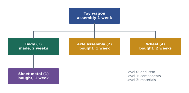
For items with dependent demand, such as components and sub-assemblies, forecasting is unnecessary: their requirements can be calculated from the MPS. Material requirements planning (MRP) uses three inputs: the MPS (what end items are needed and when), the bill of materials (BOM), which lists the components and quantities needed to make each item in a hierarchical product structure, and inventory records, which show on-hand quantities, scheduled receipts and lead times. MRP works down the BOM level by level, calculating gross requirements, subtracting available inventory to get net requirements and offsetting each planned order by its lead time to determine when it must be released.
Worked problem
An MRP calculation for wheels
A toy maker's MPS calls for 200 wagons to be completed in week 6 and 150 in week 8. Final assembly takes one week. Each wagon needs 4 wheels, which are bought with a two-week lead time; 300 wheels are on hand and none are on order. Wheels are ordered lot-for-lot (exactly the net requirement). When and how many wheels should be ordered?
Show solution
- Wagon assembly must start one week before completion: 200 in week 5 and 150 in week 7.
- Gross requirements for wheels: 4 × 200 = 800 in week 5; 4 × 150 = 600 in week 7.
- Week 5 net requirement = 800 − 300 on hand = 500; week 7 net requirement = 600 (no stock left).
- Offsetting by the two-week lead time: release an order for 500 wheels in week 3 and 600 wheels in week 5.
Answer: Planned order releases are 500 wheels in week 3 and 600 in week 5. Each component in the BOM is calculated the same way, level by level.
| Week | 1 | 2 | 3 | 4 | 5 | 6 | 7 | 8 |
|---|---|---|---|---|---|---|---|---|
| Gross requirements | 800 | 600 | ||||||
| Projected on hand (300 at start) | 300 | 300 | 300 | 300 | 0 | 0 | 0 | 0 |
| Net requirements | 500 | 600 | ||||||
| Planned order receipts | 500 | 600 | ||||||
| Planned order releases | 500 | 600 |
MRP systems also choose lot sizes (lot-for-lot, fixed quantities, EOQ-based or period-order quantities), generate capacity requirements plans that load planned orders onto work centers, and issue exception messages when dates must change. Their weakness is that they assume lead times are fixed and capacity is unlimited; if planned orders exceed what a work center can do, the plan is infeasible. Capacity requirements planning and finite-capacity scheduling address this, and planners must keep lead times, BOMs and inventory records accurate, because MRP magnifies data errors.
ERP and digital planning systems
Manufacturing resource planning (MRP II) extended MRP to include capacity, finance and marketing. Enterprise resource planning (ERP) systems integrate data and processes across the whole organization (finance, human resources, procurement, sales, production, inventory and distribution) in a single database, so that a sales order automatically updates the production plan, material requirements, purchase orders and financial forecasts. Major vendors offer cloud-based systems, and smaller firms use simpler cloud ERP packages. ERP implementations are notoriously difficult and expensive; failures usually stem less from software than from poor data, unclear processes and inadequate change management.
Advanced planning and scheduling (APS) systems add optimization and finite-capacity logic on top of ERP data, and many now use machine learning to improve forecasts and suggest schedule changes. Distribution requirements planning (DRP) applies MRP logic to multi-level distribution networks. Digital twins, virtual models of a plant or supply chain fed with live data, let planners test what-if scenarios before committing.
Scheduling and sequencing
Short-term scheduling decides which jobs to run on which resources and in what order. Loading assigns jobs to work centers; sequencing decides the order in which jobs waiting at a work center are processed. Gantt charts, named after Henry Gantt, show jobs or resources against a time axis and are still widely used, now in software. Forward scheduling starts as soon as a job is received and works forward to find the earliest completion date; backward scheduling starts from the due date and works back to find the latest start date, which supports just-in-time operations.
Priority rules for sequencing jobs at a single work center include first come, first served (FCFS), shortest processing time (SPT), earliest due date (EDD), longest processing time (LPT) and critical ratio (CR), which is time remaining until the due date divided by processing time remaining; jobs with the lowest ratio go first. Each rule optimizes different measures. SPT minimizes average completion time and average work in process; EDD tends to minimize maximum lateness; FCFS is perceived as fair, especially where customers are present. No rule is best on every measure, so the choice depends on what matters most.
# Sequencing five jobs at one machine with four priority rules (times in days)
jobs = {"A": (6, 8), "B": (2, 6), "C": (8, 18), "D": (3, 15), "E": (9, 23)}  # (processing, due)
def evaluate(order):
    t = flow = late = tardy = 0
    for j in order:
        p, due = jobs[j]
        t += p; flow += t
        late += max(t - due, 0); tardy += t > due
    n = len(order)
    return flow / n, late / n, tardy
rules = {
    "FCFS": list(jobs),
    "SPT": sorted(jobs, key=lambda j: jobs[j][0]),
    "EDD": sorted(jobs, key=lambda j: jobs[j][1]),
    "LPT": sorted(jobs, key=lambda j: -jobs[j][0]),
}
print("rule  sequence    avg completion  avg lateness  late jobs")
for r, order in rules.items():
    f, l, k = evaluate(order)
print(f"{r:<5} {'-'.join(order):<11} {f:>14.1f} {l:>13.1f} {k:>10}")rule sequence avg completion avg lateness late jobs FCFS A-B-C-D-E 15.4 2.2 3 SPT B-D-A-C-E 13.0 1.8 3 EDD B-A-D-C-E 13.6 1.2 2 LPT E-C-A-D-B 20.6 9.6 3
For these five jobs, SPT gives the lowest average completion time (13.0 days), EDD gives the lowest average lateness and the fewest late jobs, and LPT performs worst on every measure. FCFS falls in between. A print shop that promises firm dates to business clients might prefer EDD; a repair shop that wants to keep the queue of waiting jobs short might prefer SPT, with a rule that no job waits beyond a set limit so long jobs are not starved.
Worked problem
Johnson's rule for two machines
Five orders at a cabinet shop must each be cut (machine 1) and then finished (machine 2). Times in hours: order P: 5 and 2; Q: 1 and 6; R: 9 and 7; S: 3 and 8; T: 10 and 4. Use Johnson's rule to minimize the total time to complete all orders.
Show solution
- Johnson's rule: find the shortest remaining time; if it is on machine 1, schedule that job as early as possible; if on machine 2, as late as possible; remove it and repeat.
- Shortest is Q on machine 1 (1 h): Q goes first. Next is P on machine 2 (2 h): P goes last.
- Next is S on machine 1 (3 h): S goes second. Next is T on machine 2 (4 h): T goes fourth (just before P).
- R fills the remaining middle position: sequence Q–S–R–T–P.
- Machine 1 finishes at 1, 4, 13, 23 and 28 hours; machine 2 finishes Q at 7, S at 15, R at 22, T at 27 and P at 30 hours.
Answer: The sequence Q–S–R–T–P completes all five orders in 30 hours, the minimum possible for this two-machine flow shop.
Scheduling services and people
Service scheduling often focuses on people rather than jobs. Workforce scheduling matches staffing to demand patterns that vary by hour and day, using the queuing models of lesson 4 to set required staff levels, then building shifts and rosters that respect labor rules, collective agreements, skills and employee preferences. Software that optimizes rosters is widespread in call centers, hospitals, airlines and retail. Appointment systems smooth demand by spreading customers over time; clinics often overbook slightly to offset no-shows, a newsvendor-style trade-off. Unpredictable 'on-call' schedules impose real costs on workers, and several jurisdictions have adopted fair scheduling or right-to-disconnect rules that planners must follow.
Common mistakes
MistakeLetting sales, operations and finance work from different plans.
InsteadUse sales and operations planning to agree one integrated plan each month.
MistakeChoosing a chase strategy without counting hiring, training and layoff costs.
InsteadCompare full costs, including quality and morale effects, of chase, level and mixed plans.
MistakeForecasting demand for components that go into planned products.
InsteadCalculate dependent demand with MRP from the MPS and bill of materials.
MistakeTrusting MRP output when records are inaccurate.
InsteadKeep BOMs, lead times and inventory records accurate; MRP magnifies errors.
MistakeExpecting one sequencing rule to be best on every measure.
InsteadChoose the rule that matches the goal: SPT for flow time, EDD for due dates.
MistakePromising delivery dates without checking available capacity.
InsteadUse available-to-promise and capacity checks before committing.
Summary and key terms
- Planning runs from long-range capacity through aggregate planning and the MPS to daily schedules.
- S&OP is a monthly cross-functional process that agrees one plan balancing demand and supply.
- Aggregate planning uses chase, level or mixed strategies, with levers such as hiring, overtime, subcontracting and inventory.
- Employment laws on notice, layoffs and overtime shape aggregate planning choices.
- The MPS sets specific end items by week; available-to-promise supports order promising.
- MRP explodes the MPS through the bill of materials, nets inventory and offsets lead times.
- ERP integrates data across functions; APS adds optimization and finite capacity.
- Sequencing rules such as SPT and EDD optimize different measures; Johnson's rule minimizes makespan for two machines.
- Service scheduling matches staff to demand while respecting labor rules and fair scheduling.
- Sales and operations planning
- A monthly process that balances demand and supply and agrees one integrated plan.
- Aggregate plan
- A medium-range plan of output, workforce and inventory for product families.
- Chase strategy
- Matching production to demand each period by changing capacity.
- Level strategy
- Keeping output constant and absorbing demand changes with inventory.
- Master production schedule
- A plan of specific end items, quantities and dates.
- Available-to-promise
- Uncommitted planned production that can be promised to new orders.
- Bill of materials
- A list of the components and quantities needed to make an item.
- Material requirements planning
- A system that calculates dependent demand and order timing from the MPS.
- Enterprise resource planning
- An integrated information system covering all business functions.
- Johnson's rule
- A method for sequencing jobs through two machines to minimize total completion time.
Practice problems
Work each problem on paper first, then reveal the answer to check.
Name the three levels of operations planning by horizon.
Show answer
Long-range, medium-range (aggregate) and short-range (MPS and scheduling).
Give one advantage and one disadvantage of a level strategy.
Show answer
Stable workforce; inventory holding cost and risk.
Why do services often use chase strategies?
Show answer
They cannot store output in inventory.
Each chair needs 4 legs; 120 chairs are due in week 6 with a 1-week assembly time; 200 legs are on hand; leg lead time is 2 weeks. When and how many legs should be ordered?
Show answer
480 − 200 = 280 legs, released in week 3.
What is available-to-promise?
Show answer
The part of planned production not yet committed to customer orders.
Jobs with times 4, 1 and 3 days: what is the SPT sequence and average completion time?
Show answer
1, 3, 4; completion times 1, 4, 8; average 4.33 days.
Which rule tends to minimize maximum lateness?
Show answer
Earliest due date (EDD).
A job is due in 6 days and needs 4 days of work. What is its critical ratio?
Show answer
1.5.
Why are ERP implementations often difficult?
Show answer
They require clean data, redesigned processes and organizational change, not just software.
Portfolio task: build a six-month chase and level plan for an organization you know and compare costs.
Show answer
Answers vary; show demand, workforce, inventory and costs.
Lesson quiz · 5 questions
Score 60% or more to complete this lesson.
Create a free account to save your progress, take quizzes and earn a certificate.