
BIOL-410 · Lesson 9 of 12 · 28 min
Transcriptomics: RNA-seq and differential expression
The genome is largely the same in every cell of an organism, but which genes are transcribed, and how much, differs between tissues, developmental stages, conditions and individual cells. Measuring the transcriptome, the set of RNA molecules present, is therefore one of the most informative experiments in biology. RNA sequencing (RNA-seq) has largely replaced microarrays for this purpose. BIOL-207 introduced the idea of normalizing read counts; this lesson covers the full workflow, the statistics of count data, the testing of thousands of genes at once, and single-cell transcriptomics.
Designing an RNA-seq experiment
An RNA-seq experiment begins long before sequencing. The biological question determines the comparison, for example drought-stressed versus watered plants, or tumor versus normal tissue, and the design must allow that comparison to be separated from everything else. The single most important design decision is the number of biological replicates: independent samples from different individuals or cultures, as opposed to technical replicates, repeated measurements of one sample. Biological variation between individuals is usually much larger than technical noise, and without replicates it cannot be estimated, so no valid test of differential expression is possible. Three replicates per group is a common minimum; studies of subtle effects or variable material such as human tissue need many more.
Confounding is the other great danger. If all control samples are extracted on Monday and all treated samples on Friday, or sequenced on different runs, any difference may reflect the batch rather than the treatment, and no analysis can separate them. Samples should be randomized across processing batches, and batches recorded so they can be modeled. Library preparation choices also matter. Messenger RNA can be enriched by capturing poly(A) tails, which gives clean mRNA profiles but loses non-polyadenylated RNAs and requires intact RNA; ribosomal RNA, typically 80 percent or more of total RNA, can instead be depleted, which retains noncoding and degraded RNA. Stranded protocols preserve which DNA strand was transcribed, resolving overlapping antisense genes.
From reads to counts
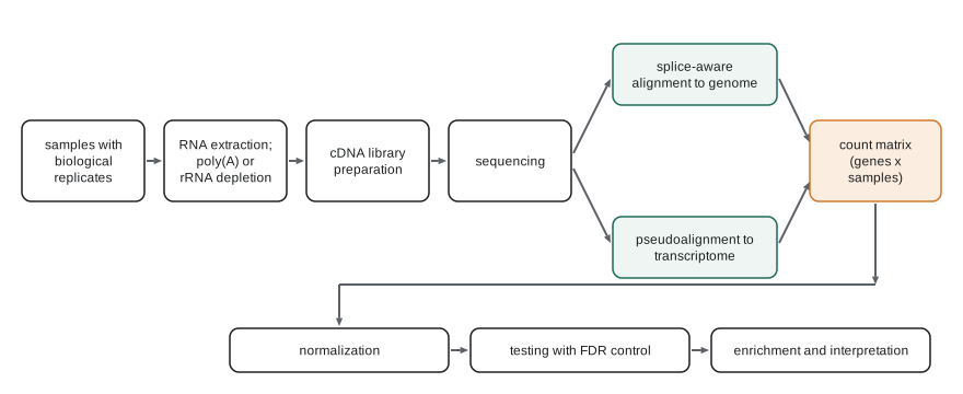
Reads from mature mRNA span exon–exon junctions, so mapping them to the genome needs a splice-aware aligner that can split a read across an intron, written in the CIGAR string with the N operation (lesson 6). STAR and HISAT2 are widely used; they discover novel junctions as well as known ones. The number of reads overlapping each gene's exons is then counted. An alternative is pseudoalignment, introduced by kallisto in 2016 and also used by salmon: instead of computing base-level alignments, the read's k-mers are matched against an index of the transcriptome to determine which transcripts it is compatible with. Because many reads are compatible with several isoforms of a gene, an expectation-maximization algorithm apportions them, estimating the abundance of each transcript. Pseudoalignment is very fast and accurate for quantifying annotated transcripts, while genome alignment is needed to discover new genes, junctions or fusion transcripts.
The result is a count matrix: genes or transcripts in rows, samples in columns, each entry the number of reads assigned. Counts are not directly comparable between samples or between genes. A sample sequenced to 40 million reads has roughly twice the counts of one sequenced to 20 million, and a long gene yields more fragments than a short gene expressed at the same molar level. Normalization addresses both.
Normalization
Counts per million (CPM) divide each count by the sample's total count and multiply by one million, correcting for sequencing depth but not gene length. RPKM and FPKM (reads or fragments per kilobase per million) also divide by gene length, but have the defect that the values in different samples sum to different totals. Transcripts per million (TPM) reverse the order: first divide each count by gene length in kilobases, giving reads per kilobase, then scale so that each sample sums to one million. TPM values can be read as the relative molar proportion of each transcript in the sample, and are comparable within a sample across genes.
Neither CPM nor TPM handles a subtler problem, composition bias. If one condition massively expresses a few genes, those genes take a larger share of the reads, and every other gene's share falls, even though its absolute expression is unchanged. Methods for differential expression therefore estimate size factors that assume most genes do not change. DESeq2's median-of-ratios method computes, for each gene, the geometric mean of its counts across all samples as a pseudo-reference; for each sample, it takes the ratio of each gene's count to that reference, and uses the median ratio as the sample's size factor. The median is unaffected by a minority of strongly changed genes. The TMM method of edgeR uses a trimmed mean of log ratios for the same purpose.
# CPM, TPM and DESeq-style median-of-ratios size factors on an invented count matrix.
import numpy as np
genes = ['geneA', 'geneB', 'geneC', 'geneD', 'geneE', 'geneF']
length_kb = np.array([1.0, 4.0, 2.0, 0.5, 3.0, 1.5])
# columns: control_1, control_2, treated_1, treated_2 (treated_2 sequenced twice as deeply)
counts = np.array([
    [500,  520,   510,  1010],
    [2000, 2100, 2050,  4150],
    [800,   780, 4000,  8100],      # strongly induced by treatment
    [100,   110,  105,   205],
    [1500, 1450, 1480,  3000],
    [600,   640,  610,  1230]], dtype=float)
cpm = counts / counts.sum(axis=0) * 1e6
rpk = counts / length_kb[:, None]
tpm = rpk / rpk.sum(axis=0) * 1e6
log_geo_mean = np.log(counts).mean(axis=1)
size = np.exp(np.median(np.log(counts) - log_geo_mean[:, None], axis=0))
norm = counts / size
np.set_printoptions(suppress=True)
print('library sizes:', counts.sum(axis=0).astype(int))
print('size factors: ', np.round(size, 2))
print(f"{'gene':6s} {'CPM c1':>8s} {'CPM t2':>8s} {'TPM c1':>8s} {'norm c1':>8s} {'norm t1':>8s} {'norm t2':>8s}")
for g, c, t, n in zip(genes, cpm, tpm, norm):
print(f"{g:6s} {c[0]:8.0f} {c[3]:8.0f} {t[0]:8.0f} {n[0]:8.0f} {n[2]:8.0f} {n[3]:8.0f}")library sizes: [ 5500 5600 8755 17695] size factors: [0.82 0.86 0.84 1.69] gene CPM c1 CPM t2 TPM c1 norm c1 norm t1 norm t2 geneA 90909 57078 200000 611 606 598 geneB 363636 234530 200000 2444 2437 2458 geneC 145455 457756 160000 977 4755 4798 geneD 18182 11585 80000 122 125 121 geneE 272727 169539 200000 1833 1759 1777 geneF 109091 69511 160000 733 725 729
Look at gene A, which the invented data were built to have unchanged expression. Its CPM falls in the treated samples, because induced gene C takes a larger share of the reads, which would wrongly suggest down-regulation. After median-of-ratios normalization, gene A's values are nearly equal across all four samples, including the deeply sequenced one, while gene C stands out with roughly fivefold induction. TPM, meanwhile, changes the comparison of genes within a sample: in control 1, long gene B has four times as many reads as gene A, but the same TPM, because it is four times longer, so the two transcripts are present in similar molar amounts.
Statistics of counts
If the same library were sequenced repeatedly, counts for a gene would vary approximately as a Poisson distribution, whose variance equals its mean. Between biological replicates, however, the true expression level itself varies, and the counts are overdispersed: their variance exceeds the mean, increasingly so for highly expressed genes. The negative binomial distribution captures this with a dispersion parameter \(\alpha\):
With only three replicates per group, estimating a separate dispersion for each gene is unreliable, so DESeq2 and edgeR share information across genes: they fit a trend of dispersion against mean expression and shrink each gene's estimate toward it. They then fit a generalized linear model for each gene, with the condition, and any batch or other covariates, as predictors, and test whether the coefficient for condition differs from zero. The limma-voom approach instead transforms counts to log-CPM with precision weights and uses linear models with moderated t statistics. These methods are well tested and generally agree on strong effects; they differ at the margins.
Testing thousands of genes
A typical experiment tests 15,000 to 20,000 genes. At a significance threshold of 0.05, even if no gene changed, about 1,000 would appear significant by chance. Controlling the family-wise error rate with the Bonferroni correction (dividing the threshold by the number of tests) is too strict for discovery. Instead, the false discovery rate (FDR), the expected proportion of false positives among the genes declared significant, is controlled with the procedure of Yoav Benjamini and Yosef Hochberg (1995): sort the \(m\) p-values, find the largest rank \(i\) with \(p_{(i)} \le (i/m)q\), and declare the first \(i\) genes significant. Equivalently, each gene gets an adjusted p-value, often called a q-value or padj, and genes with padj below 0.05 or 0.1 are reported.
# Simulate negative binomial counts, test each gene on log-scale normalized values, and control the FDR.
import numpy as np
from scipy import stats
rng = np.random.default_rng(410)
n_genes, n_rep = 4000, 4
base = rng.lognormal(mean=5, sigma=1.2, size=n_genes)
true_lfc = np.zeros(n_genes)
changed = rng.choice(n_genes, 300, replace=False)
true_lfc[changed] = rng.choice([-1, 1], 300) * rng.uniform(1, 2.5, 300)
alpha = 0.05 + 1.0 / base
def nb(mu):
    n = 1 / alpha[:, None]
    return rng.negative_binomial(n, n / (n + mu))
ctrl = nb(np.repeat(base[:, None], n_rep, axis=1))
trt = nb(np.repeat((base * 2 ** true_lfc)[:, None], n_rep, axis=1))
counts = np.hstack([ctrl, trt]).astype(float)
keep = counts.mean(axis=1) >= 10                          # filter very low counts
logc = np.log2(counts / counts.sum(axis=0) * 1e6 + 1)
t, p = stats.ttest_ind(logc[:, n_rep:], logc[:, :n_rep], axis=1)
p = np.where(keep, p, 1.0)
order = np.argsort(p)
m = keep.sum()
ranked = p[order] * m / np.arange(1, len(p) + 1)
padj = np.empty_like(p)
padj[order] = np.minimum(1, np.minimum.accumulate(ranked[::-1])[::-1])
sig = padj < 0.05
is_true = true_lfc != 0
print(f"genes tested {m}, truly changed {is_true.sum()}")
print(f"raw p < 0.05: {(p < 0.05).sum()} genes, of which false {((p < 0.05) & ~is_true).sum()}")
print(f"BH padj < 0.05: {sig.sum()} genes, of which false {(sig & ~is_true).sum()} "
f"(observed FDR {(sig & ~is_true).sum() / max(sig.sum(), 1):.1%}), recovered {(sig & is_true).sum()} of {is_true.sum()}")genes tested 3934, truly changed 300 raw p < 0.05: 520 genes, of which false 233 BH padj < 0.05: 245 genes, of which false 15 (observed FDR 6.1%), recovered 230 of 300
Without correction, the list of genes with p below 0.05 contains more than two hundred false positives, nearly half the list; with the Benjamini–Hochberg adjustment, the observed false discovery proportion is close to the nominal 5 percent, at the cost of missing some true changes, mostly those with small fold changes in low-count genes. (The example tests log-scale values with t tests for simplicity; with real data, a negative binomial method such as DESeq2 would be preferred, especially with few replicates.)
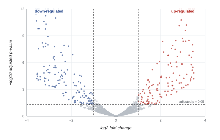
Results are commonly displayed as a volcano plot, with the log2 fold change on the horizontal axis and the negative log10 of the p-value on the vertical axis, so that genes with large and significant changes lie in the upper corners. Fold changes estimated from few, noisy counts are inflated, so modern methods shrink log fold changes toward zero when evidence is weak, which makes ranking by effect size more reliable.
Interpreting gene lists
A list of several hundred differentially expressed genes is hard to interpret one gene at a time. Over-representation analysis asks whether genes annotated to a Gene Ontology term or pathway (lesson 8) appear in the list more often than expected by chance, using the hypergeometric distribution or Fisher's exact test, with the background set to all genes that were tested, not the whole genome. Gene set enrichment analysis (GSEA) instead ranks all genes by their change and asks whether a set's members cluster toward the top or bottom of the ranking, which detects coordinated modest changes. Enrichment results depend on annotation quality and on many correlated tests, so they suggest hypotheses rather than prove mechanisms.
Single-cell RNA-seq
Bulk RNA-seq measures the average of millions of cells, hiding differences between cell types and states. Single-cell RNA-seq (scRNA-seq) captures individual cells, most commonly in droplet systems that encapsulate each cell with a bead carrying oligonucleotides that include a cell barcode, a unique molecular identifier (UMI) and a poly(T) capture sequence. After sequencing, reads are assigned to cells by barcode, and UMIs are counted to give molecule counts per gene per cell. Tens of thousands of cells can be profiled in one experiment, but each cell yields only a few thousand molecules, so the data are sparse, with most entries zero.
Analysis follows a standard path. Quality control removes empty droplets, doublets (two cells in one droplet) and damaged cells, often identified by a high fraction of mitochondrial transcripts. Counts are normalized and log-transformed, highly variable genes are selected, and principal component analysis reduces the data to tens of dimensions. Cells are clustered, usually by building a graph of nearest neighbors in principal component space and applying a community detection algorithm such as Leiden, and visualized in two dimensions with UMAP or t-SNE. Clusters are labeled as cell types using marker genes. Two-dimensional embeddings distort distances, so cluster positions and sizes on a UMAP plot should not be over-interpreted. Large efforts such as the Human Cell Atlas are building reference maps of all cell types in the human body.
# Synthetic single-cell counts for three cell types: normalize, reduce with PCA and cluster with k-means.
import numpy as np
rng = np.random.default_rng(3)
n_genes, sizes = 300, (150, 100, 60)
base = rng.gamma(0.6, 1.5, n_genes)
programs = []
for t in range(3):
    prog = base.copy()
    markers = rng.choice(n_genes, 20, replace=False)
    prog[markers] *= rng.uniform(4, 10, 20)
    programs.append(prog)
labels = np.repeat([0, 1, 2], sizes)
depth = rng.lognormal(0, 0.4, len(labels))
X = rng.poisson(np.array([programs[t] for t in labels]) * depth[:, None])
print(f"cells {X.shape[0]}, genes {X.shape[1]}, zero entries {np.mean(X == 0):.0%}")
Xn = np.log1p(X / X.sum(axis=1, keepdims=True) * 1e4)
Xc = Xn - Xn.mean(axis=0)
U, S, Vt = np.linalg.svd(Xc, full_matrices=False)
pcs = U[:, :10] * S[:10]
print('variance explained by PC1-PC3:', np.round(S[:3] ** 2 / (S ** 2).sum(), 3))
best = None
for restart in range(5):
    cent = pcs[rng.choice(len(pcs), 3, replace=False)]
    for _ in range(50):
        assign = np.argmin(((pcs[:, None, :] - cent[None]) ** 2).sum(-1), axis=1)
        cent = np.array([pcs[assign == j].mean(0) if np.any(assign == j) else cent[j] for j in range(3)])
    inertia = ((pcs - cent[assign]) ** 2).sum()
    if best is None or inertia < best[0]:
        best = (inertia, assign)
assign = best[1]
for j in range(3):
    members = labels[assign == j]
print(f"cluster {j}: {len(members)} cells, composition by true type {np.bincount(members, minlength=3)}")cells 310, genes 300, zero entries 56% variance explained by PC1-PC3: [0.065 0.037 0.035] cluster 0: 60 cells, composition by true type [ 0 0 60] cluster 1: 100 cells, composition by true type [ 0 100 0] cluster 2: 150 cells, composition by true type [150 0 0]
Despite the sparsity, with most entries zero, the clusters recover the three cell types almost perfectly, because each type's marker genes shift its cells consistently in principal component space. Real data add continuous states, rare cell types, batch effects between samples and doublets, which make clustering and annotation more demanding.
| Approach | Measures | Strengths | Limitations |
|---|---|---|---|
| Bulk short-read RNA-seq | Average gene or transcript abundance | Mature statistics, low cost, many replicates | Hides cell-type differences; isoforms inferred |
| Long-read RNA-seq | Full-length isoforms | Direct isoform structure, fusion transcripts | Lower throughput for quantification |
| Single-cell RNA-seq | Expression per cell | Cell types, states and trajectories | Sparse data, dissociation artifacts, cost per sample |
| Spatial transcriptomics | Expression with tissue location | Cell neighborhoods and tissue architecture | Resolution and gene coverage trade-offs |
Worked problem
Diagnosing a suspicious experiment
An invented study compares liver tissue from four mice fed a high-fat diet with four on a normal diet. A principal component analysis of normalized counts shows PC1 separating samples 1 to 4 of each group from samples 5 to 8, rather than separating diets. The laboratory notebook shows that samples 1 to 4 were extracted in March and 5 to 8 in June. What happened and what should be done?
Show solution
- The strongest source of variation is the extraction date, a batch effect, not diet.
- Because each batch contains both diets, diet and batch are not confounded; the design is balanced.
- Include batch as a covariate in the model (for example, design ~ batch + diet in DESeq2), so the diet effect is estimated within batches.
- Check PCA after removing batch effects for visualization only; do not test on batch-corrected values.
- Had all high-fat samples been extracted in March and all controls in June, diet and batch would be confounded and no analysis could separate them.
Answer: A batch effect; model batch as a covariate, which is possible because the design is balanced.
Common mistakes
MistakeRunning an experiment without biological replicates.
InsteadBiological variation cannot be estimated without replicates, so differential expression cannot be tested.
MistakeComparing raw counts or CPM across conditions when a few genes change massively.
InsteadUse size factors such as median-of-ratios or TMM that correct for composition bias.
MistakeComparing TPM of one gene across conditions as if absolute.
InsteadTPM is a within-sample proportion; differential testing should use counts with proper normalization.
MistakeReporting genes with raw p < 0.05 from thousands of tests.
InsteadControl the false discovery rate with Benjamini–Hochberg or a similar method.
MistakeReading biological meaning into distances on a UMAP plot.
InsteadEmbeddings distort distances; use them for visualization and rely on clustering and markers for conclusions.
Summary and key terms
- Good RNA-seq design depends on biological replicates, randomization across batches and appropriate library choices.
- Splice-aware aligners map reads across introns; pseudoalignment quantifies transcripts rapidly with expectation maximization.
- CPM corrects for depth, TPM for depth and length within samples, and median-of-ratios or TMM size factors for composition bias.
- Counts are overdispersed and modeled with the negative binomial; dispersion estimates are shared across genes.
- Benjamini–Hochberg controls the false discovery rate across thousands of tests; volcano plots and enrichment analyses aid interpretation.
- Single-cell RNA-seq uses barcodes and UMIs; analysis involves QC, normalization, PCA, graph clustering and marker-based annotation.
- biological replicate
- An independent sample from a different individual or culture.
- batch effect
- Systematic variation caused by processing differences rather than biology.
- pseudoalignment
- Determining which transcripts a read is compatible with by k-mer matching, without base-level alignment.
- TPM
- Transcripts per million: length-normalized counts scaled to sum to one million per sample.
- size factor
- A per-sample scaling factor used to normalize counts for depth and composition.
- overdispersion
- Variance in counts greater than the mean, as between biological replicates.
- negative binomial distribution
- A count distribution with variance μ + αμ², used for RNA-seq data.
- false discovery rate
- The expected proportion of false positives among results declared significant.
- volcano plot
- A plot of fold change against significance for all tested genes.
- cell barcode
- A sequence tag identifying the cell of origin of reads in single-cell sequencing.
Practice problems
Work each problem on paper first, then reveal the answer to check.
Why are technical replicates not a substitute for biological replicates?
Show answer
They measure only technical noise, not the variation between individuals that tests must account for.
Gene X has 300 reads and length 3 kb; gene Y 100 reads and length 1 kb in the same sample. How do their TPMs compare?
Show answer
Equal: both have 100 reads per kilobase.
Why does the median-of-ratios method use the median?
Show answer
It is robust to a minority of strongly changed genes.
With mean 100 and dispersion 0.1, what is the negative binomial variance?
Show answer
100 + 0.1 x 10,000 = 1,100.
Ten genes have sorted p-values 0.001, 0.004, 0.012, 0.03, 0.2 ... from 10 tests. With q = 0.05, which pass Benjamini–Hochberg?
Show answer
Thresholds are 0.005, 0.01, 0.015, 0.02: the first three pass (0.012 ≤ 0.015) but 0.03 > 0.02, so three genes.
What background set should over-representation analysis use?
Show answer
All genes tested (expressed and filtered) in the experiment.
What does a high mitochondrial read fraction indicate in single-cell data?
Show answer
A damaged or dying cell whose cytoplasmic RNA leaked out.
Why can pseudoalignment not discover new splice junctions?
Show answer
It matches reads only against an index of known transcripts.
Lesson quiz · 5 questions
Score 60% or more to complete this lesson.
Create a free account to save your progress, take quizzes and earn a certificate.