
BIOL-410 · Lesson 7 of 12 · 27 min
Variants: calling, formats and interpretation
Once reads are mapped, the differences between them and the reference can be identified. Some differences are sequencing or mapping errors; others are genuine variants carried by the sample. Variant calling is the statistical problem of telling them apart and assigning genotypes, and it underlies clinical diagnosis, cancer genomics, population genetics (BIOL-322) and outbreak tracking. This lesson covers the kinds of variants, the probability model behind genotype calling, the VCF format, filtering and benchmarking, somatic and structural variants, and how variants are annotated and interpreted.
Kinds of variants
Single-nucleotide variants (SNVs) change one base; in a population context, common SNVs are called single-nucleotide polymorphisms (SNPs). Two unrelated human genomes differ at about 4 to 5 million sites, most of them SNVs. Small insertions and deletions (indels) of up to about 50 bases are the next most common; in coding sequence, indels whose length is not a multiple of three shift the reading frame. Structural variants (SVs) are larger: deletions, duplications and other copy-number variants, insertions including mobile elements such as Alu and LINE-1 insertions, inversions and translocations. Although fewer in number, SVs affect more bases per genome than SNVs, and long-read studies have shown that each human genome carries more than 20,000 of them. Tandem repeat expansions, such as the CAG repeats of Huntington disease, form a further class that short reads struggle to measure.
A typical germline short-read pipeline follows a sequence of steps standardized by the Broad Institute's GATK Best Practices: map reads, mark duplicates, optionally recalibrate base quality scores using known variant sites, call variants per sample, combine samples by joint genotyping, and filter. Each step addresses a specific source of error, and each makes assumptions worth knowing.
The pileup and genotype likelihoods
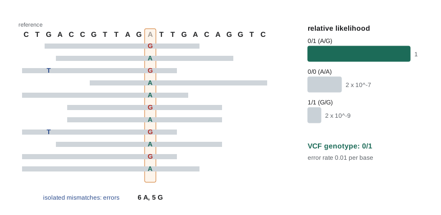
At each position, the bases of all reads covering it form a pileup. Suppose a diploid individual has, at some position, reference allele A and possible alternative G. The genotype is AA, AG or GG. If each base call has error probability \(e\), then a read from a chromosome carrying A shows A with probability \(1 - e\), and a heterozygote's reads come from either chromosome with probability one half. For \(n\) reads of which \(k\) show G, the likelihood of each genotype is:
(the heterozygous case is exact when errors are ignored, and close otherwise; the per-read formula \((1-e)/2 + e/2\) gives one half per read in a two-allele model). Real callers use each base's own quality score in place of a single \(e\). Combining the likelihoods with prior probabilities of each genotype, which reflect that most positions are homozygous for the reference allele, gives posterior probabilities by Bayes' theorem. The called genotype is the most probable, and its confidence is expressed as a Phred-scaled genotype quality (GQ) from the probability that it is wrong. The likelihoods themselves are stored, normalized and Phred-scaled, as PL values.
# Diploid genotype likelihoods, posteriors and genotype quality from allele counts in a pileup.
import math
def call(n_ref, n_alt, err=0.01, prior=(0.998, 0.0015, 0.0005)):
    lik = {
        '0/0': (1 - err) ** n_ref * err ** n_alt,
        '0/1': 0.5 ** (n_ref + n_alt),
        '1/1': err ** n_ref * (1 - err) ** n_alt,
    }
    post = {g: lik[g] * p for g, p in zip(lik, prior)}
    z = sum(post.values())
    post = {g: v / z for g, v in post.items()}
    best = max(post, key=post.get)
    p_wrong = max(1 - post[best], 1e-30)
    gq = min(99, int(-10 * math.log10(p_wrong)))
    pl_raw = {g: -10 * math.log10(max(v, 1e-300)) for g, v in lik.items()}
    m = min(pl_raw.values())
    pl = ','.join(str(round(pl_raw[g] - m)) for g in ('0/0', '0/1', '1/1'))
    return best, gq, pl

for n_ref, n_alt in [(30, 0), (29, 1), (15, 14), (3, 2), (1, 28), (6, 1), (9, 3)]:
    gt, gq, pl = call(n_ref, n_alt)
print(f"ref {n_ref:2d} alt {n_alt:2d}: GT {gt} GQ {gq:2d} PL {pl}")ref 30 alt 0: GT 0/0 GQ 99 PL 0,89,599 ref 29 alt 1: GT 0/0 GQ 97 PL 0,69,559 ref 15 alt 14: GT 0/1 GQ 99 PL 193,0,213 ref 3 alt 2: GT 0/0 GQ 4 PL 25,0,45 ref 1 alt 28: GT 1/1 GQ 61 PL 539,66,0 ref 6 alt 1: GT 0/0 GQ 29 PL 0,1,100 ref 9 alt 3: GT 0/0 GQ 5 PL 24,0,144
The examples show why depth matters. One alternative read among 30 is almost certainly an error. Fifteen and fourteen reads give a confident heterozygote. With three and two reads, or nine and three, the likelihoods favor a heterozygote (the zero in the middle of the PL values), but the prior, which says that almost every position is homozygous reference, pulls the posterior back to 0/0 with a genotype quality of only 4 or 5: the site is genuinely uncertain. Six reference reads with one alternative read are called homozygous reference with modest confidence, yet a heterozygote would produce such counts not very rarely. Real callers use priors informed by population data, so a site known to be polymorphic is treated differently from a random position. Low-coverage sites are therefore uncertain, and whether a site was confidently called homozygous reference or simply not covered is important information, which is why per-sample genomic VCF (gVCF) files record confidence for non-variant blocks too.
Modern callers go beyond independent pileup columns. GATK HaplotypeCaller, when it finds evidence of variation in a region, reassembles the reads locally into candidate haplotypes with a de Bruijn graph, aligns each read to each haplotype with a pair hidden Markov model, and computes genotype likelihoods from those alignments; this handles indels and nearby variants much better than column-by-column counting. DeepVariant, released by Google in 2018, turns the pileup around each candidate into an image-like tensor and uses a convolutional neural network to classify the genotype, learning error patterns directly from data with known truth. Both are widely used, and DeepVariant models trained for long reads have helped make long-read variant calling routine.
The VCF format
Variants are stored in the Variant Call Format (VCF). Header lines beginning with ## define the reference, the meaning of each INFO and FORMAT field and the filters applied; a line beginning with #CHROM names the columns. Each data line gives the chromosome, the 1-based position, an identifier such as a dbSNP rs number, the reference and alternative alleles, a Phred-scaled variant quality, the filter status (PASS or the names of failed filters), site-level INFO annotations, and then for each sample a FORMAT-defined list such as genotype, allelic depths, total depth, genotype quality and likelihoods.
| Column | Example | Meaning |
|---|---|---|
| CHROM | chr17 | Chromosome |
| POS | 43,092,919 | 1-based position of the first REF base |
| ID | rs80357713 | Identifier, or . if none |
| REF / ALT | C / T | Reference and alternative alleles; indels include the preceding base |
| QUAL | 812.4 | Phred-scaled probability that the site is not variant |
| FILTER | PASS | Filters passed, or names of failed filters |
| INFO | DP=58;AF=0.5 | Site annotations such as depth and allele frequency |
| FORMAT / sample | GT:AD:DP:GQ:PL / 0/1:30,28:58:99:812,0,901 | Genotype, allelic depths, depth, genotype quality, likelihoods |
Genotypes are written with allele indexes: 0 for the reference, 1 for the first alternative, and so on; a slash marks unphased genotypes (0/1) and a vertical bar phased ones (0|1), in which the left allele is on one known haplotype. The same indel can be written in several ways in a repetitive context, for example deleting any one of four Ts in TTTT, so variants are normalized, left-aligned and trimmed to a minimal representation, before databases are compared.
Filtering and benchmarking
Raw calls contain artifacts. Common filters examine strand bias (alternative allele seen only on reads from one strand, a sign of an artifact), low mapping quality of supporting reads, a low ratio of quality to depth, extreme depth (often a collapsed repeat), allele balance far from 50 percent for a supposed heterozygote, and clustering of variants. Hard filters set thresholds on such annotations; machine-learning filters train on known true and false variants. The transition to transversion ratio, about 2.0 to 2.1 for genome-wide human SNVs and higher in exons, is a quick check: random errors give a ratio near 0.5, so a low ratio indicates many false calls.
Accuracy is measured against benchmark truth sets. The Genome in a Bottle Consortium, hosted by the US National Institute of Standards and Technology (NIST), characterizes reference samples, including the HG002 son of an Ashkenazi Jewish trio, with many technologies and publishes high-confidence variant calls for defined regions. Pipelines are scored by precision (the fraction of called variants that are true), recall or sensitivity (the fraction of true variants called) and their harmonic mean, F1. Leading short-read pipelines exceed 99.5 percent F1 for SNVs in easy regions, with lower accuracy for indels and in difficult regions such as segmental duplications.
# Parse invented VCF lines, apply simple filters, compute Ti/Tv and benchmark against a truth set.
vcf = """chr1\t1001\t.\tA\tG\t500\t.\tDP=40;SB=0.02\tGT:AD\t0/1:21,19
chr1\t1550\t.\tC\tT\t620\t.\tDP=38;SB=0.05\tGT:AD\t0/1:18,20
chr1\t2210\t.\tG\tT\t35\t.\tDP=60;SB=0.97\tGT:AD\t0/1:52,8
chr1\t3120\t.\tT\tC\t900\t.\tDP=35;SB=0.10\tGT:AD\t1/1:0,35
chr1\t4400\t.\tC\tA\t28\t.\tDP=6;SB=0.40\tGT:AD\t0/1:4,2
chr1\t5012\t.\tA\tG\t710\t.\tDP=44;SB=0.08\tGT:AD\t0/1:22,22
chr1\t6105\t.\tG\tA\t480\t.\tDP=210;SB=0.30\tGT:AD\t0/1:150,60
chr1\t7333\t.\tT\tG\t40\t.\tDP=30;SB=0.91\tGT:AD\t0/1:26,4"""
truth = {('chr1', 1001), ('chr1', 1550), ('chr1', 3120), ('chr1', 5012), ('chr1', 8100)}
transitions = {frozenset('AG'), frozenset('CT')}
kept, ti, tv = [], 0, 0
for line in vcf.splitlines():
    f = line.split('\t')
    info = dict(kv.split('=') for kv in f[7].split(';'))
    ref_d, alt_d = map(int, f[9].split(':')[1].split(','))
    reasons = []
    if float(f[5]) < 50: reasons.append('LowQual')
    if float(info['SB']) > 0.9: reasons.append('StrandBias')
    if int(info['DP']) > 150: reasons.append('HighDepth')
    if f[9].startswith('0/1') and alt_d / (ref_d + alt_d) < 0.2: reasons.append('AlleleBalance')
    print(f"{f[0]}:{f[1]} {f[3]}>{f[4]} FILTER={';'.join(reasons) or 'PASS'}")
    if not reasons:
        kept.append((f[0], int(f[1])))
        if frozenset((f[3], f[4])) in transitions: ti += 1
        else: tv += 1
tp = len(set(kept) & truth)
prec, rec = tp / len(kept), tp / len(truth)
print(f"PASS calls {len(kept)}, Ti/Tv {ti}/{tv}, precision {prec:.2f}, recall {rec:.2f}, F1 {2 * prec * rec / (prec + rec):.2f}")chr1:1001 A>G FILTER=PASS chr1:1550 C>T FILTER=PASS chr1:2210 G>T FILTER=LowQual;StrandBias;AlleleBalance chr1:3120 T>C FILTER=PASS chr1:4400 C>A FILTER=LowQual chr1:5012 A>G FILTER=PASS chr1:6105 G>A FILTER=HighDepth chr1:7333 T>G FILTER=LowQual;StrandBias;AlleleBalance PASS calls 4, Ti/Tv 4/0, precision 1.00, recall 0.80, F1 0.89
Somatic and structural variants
Cancer genomes carry somatic mutations acquired during the life of the tumor's cell lineage. Somatic calling compares a tumor sample with a matched normal sample from the same person, usually blood, so that germline variants can be excluded. It differs from germline calling because a somatic variant need not be present at 50 or 100 percent of reads: its variant allele fraction (VAF) depends on tumor purity, copy number and whether the mutation is in all tumor cells (clonal) or a subset (subclonal). A clonal heterozygous mutation in a tumor sample of 40 percent purity, with no copy-number change, is expected at a VAF of about 20 percent; subclonal mutations may be at a few percent, requiring deep sequencing. Tools such as Mutect2 model these fractions explicitly and use panels of normal samples to remove recurrent artifacts. Liquid biopsy, sequencing circulating tumor DNA in blood plasma, pushes detection to fractions below 0.1 percent, using UMIs and error-corrected sequencing.
Structural variants are detected from several signals: read depth (deletions reduce it, duplications increase it), discordant read pairs (mates mapping too far apart, too close, or in the wrong orientation), split reads (a read aligned in two parts across a breakpoint) and, with long reads, alignments that directly span the event or assemblies that contain it. Short-read SV calling has modest sensitivity, especially for insertions and in repeats, while long-read methods detect most SVs. Copy-number variants are also detected by chromosomal microarrays, still a first-line clinical test for developmental disorders in many places.
Annotation and interpretation
Variant annotation tools such as Ensembl's Variant Effect Predictor and SnpEff report each variant's location relative to genes and its predicted consequence: synonymous, missense, nonsense (stop-gained), frameshift, splice-site, regulatory or intergenic. Further annotation adds population frequency from resources such as gnomAD, the Genome Aggregation Database, whose version 4 combines exomes and genomes from more than 800,000 people; conservation scores; computational predictions of deleteriousness; and previous reports in databases such as ClinVar. A variant common in a healthy population is unlikely to cause a rare severe disease; a novel frameshift in a gene known to cause the patient's condition is a strong candidate.
Clinical classification follows the 2015 standards of the American College of Medical Genetics and Genomics and the Association for Molecular Pathology (ACMG/AMP), which combine weighted criteria (population data, computational predictions, functional evidence, segregation in families, de novo occurrence) into five classes: pathogenic, likely pathogenic, uncertain significance, likely benign and benign. Many variants are classified as variants of uncertain significance (VUS), which should not guide medical management; reclassification as evidence accumulates is common, and laboratories increasingly share classifications through ClinVar to resolve conflicts.
In the United States, clinical laboratories reporting results for patient care must be certified under the Clinical Laboratory Improvement Amendments (CLIA), and many are also accredited by the College of American Pathologists. The ACMG/AMP framework is the dominant standard, ClinVar is maintained by NCBI, and the NIH-funded Clinical Genome Resource (ClinGen) curates gene–disease validity and expert variant classifications.
Worked problem
Interpreting allele fractions in a tumor
A tumor sample estimated at 60 percent purity has a TP53 missense variant at VAF 0.31 and a KRAS variant at VAF 0.08, both in diploid regions; the matched normal shows neither. Interpret.
Show solution
- Absence in the normal sample indicates both are somatic.
- A clonal heterozygous mutation in a diploid region is expected at VAF = purity / 2 = 0.30.
- TP53 at 0.31 matches this expectation, so it is probably clonal, present in essentially all tumor cells, consistent with an early event.
- KRAS at 0.08 corresponds to about 0.08 / 0.30 ≈ 27 percent of tumor cells, so it is probably subclonal, arising later in one part of the tumor.
- Check depth: at 300-fold coverage, 0.08 is about 24 supporting reads, well above error levels; at 30-fold it would be only 2 or 3 reads and much less certain.
Answer: TP53 is likely clonal and KRAS subclonal; confidence depends on depth and purity estimates.
Common mistakes
MistakeTreating a site with no variant call as confidently reference.
InsteadIt may be uncovered or poorly covered; gVCF confidence blocks distinguish the two.
MistakeComparing indels between call sets without normalization.
InsteadLeft-align and trim indels so equivalent representations match.
MistakeExpecting somatic variants at 50 percent allele fraction.
InsteadSomatic VAF depends on purity, copy number and clonality.
MistakeActing on a variant of uncertain significance as if pathogenic.
InsteadVUS should not guide management; seek more evidence and allow reclassification.
MistakeAssuming short reads find most structural variants.
InsteadShort-read SV sensitivity is modest, especially for insertions and in repeats; long reads detect far more.
Summary and key terms
- Variants include SNVs, indels, structural variants and repeat expansions; each human genome differs from the reference at about 4 to 5 million sites.
- Genotype likelihoods from base qualities, combined with priors, give posterior genotypes, GQ and PL values.
- HaplotypeCaller reassembles local haplotypes and DeepVariant classifies pileups with a neural network.
- VCF stores sites and genotypes; indels must be normalized before comparison.
- Filters address strand bias, mapping quality, depth and allele balance; Genome in a Bottle truth sets measure precision, recall and F1.
- Somatic calling uses tumor–normal pairs and models allele fractions; interpretation combines annotation, population frequency and the ACMG/AMP classes.
- single-nucleotide variant
- A difference of one base relative to a reference.
- indel
- A small insertion or deletion.
- structural variant
- A genomic rearrangement of about 50 bases or more, such as a deletion, duplication, inversion or translocation.
- pileup
- The stack of read bases aligned at each reference position.
- genotype likelihood
- The probability of the observed reads given a particular genotype.
- genotype quality
- A Phred-scaled probability that the called genotype is wrong.
- VCF
- Variant Call Format, a text format for variant sites and sample genotypes.
- transition/transversion ratio
- The ratio of purine–purine or pyrimidine–pyrimidine changes to purine–pyrimidine changes, used as a quality check.
- variant allele fraction
- The fraction of reads at a site that carry the alternative allele.
- variant of uncertain significance
- A variant with insufficient evidence to classify as pathogenic or benign.
Practice problems
Work each problem on paper first, then reveal the answer to check.
With error rate 0.01, what is the likelihood of 10 reference reads and no alternative reads under genotype 1/1?
Show answer
0.01^10 = 10^−20.
Why do low-coverage heterozygous sites risk being called homozygous?
Show answer
By chance, few or no reads may sample the alternative allele.
What does the genotype 1|0 indicate?
Show answer
A phased heterozygote with the alternative allele on the first haplotype.
A call set has Ti/Tv of 0.9 genome-wide. What does that suggest?
Show answer
Many false-positive calls, since random errors give a ratio near 0.5 and true human SNVs about 2.
A pipeline calls 1,000 variants of which 950 are true; the truth set has 1,000 variants. Give precision, recall and F1.
Show answer
Precision 0.95, recall 0.95, F1 0.95.
What VAF is expected for a clonal heterozygous mutation at 80 percent purity in a diploid region?
Show answer
0.40.
Name three signals used to detect structural variants from short reads.
Show answer
Read depth, discordant read pairs and split reads.
Why is a variant found in 2 percent of healthy people unlikely to cause a rare severe childhood disease?
Show answer
Its population frequency is far higher than the disease frequency allows.
Lesson quiz · 5 questions
Score 60% or more to complete this lesson.
Create a free account to save your progress, take quizzes and earn a certificate.