
BIOL-410 · Lesson 3 of 12 · 26 min
Read processing, k-mers and coverage
Raw reads are never analyzed as they come off the instrument. They are checked for quality, trimmed of adapters and poor-quality ends, screened for contamination, and summarized in ways that reveal properties of the genome before any assembly or mapping is done. This lesson covers those first steps and two ideas that run through the rest of the course: coverage, the number of reads covering each position, and k-mers, the short words of fixed length into which reads can be broken. Counting k-mers, it turns out, lets you estimate a genome's size, heterozygosity and repeat content from raw reads alone.
Quality control
Quality control tools such as FastQC summarize a set of reads with a standard series of plots, and experienced analysts read them like a clinician reads a chart. The per-position quality plot shows how base quality changes along the read; a gentle decline toward the 3' end is normal for Illumina data, but a sudden drop across all reads suggests an instrument problem. The GC content distribution should be roughly normal around the genome's expected value; a second peak suggests contamination with another organism. Adapter content rises toward read ends when inserts are shorter than the read length, so the sequencer reads through the insert into the adapter. Overrepresented sequences may be adapter dimers, rRNA in an RNA-seq library, or a highly expressed gene. Duplication levels reflect library complexity: low-input libraries yield many duplicates.
None of these plots is a pass or fail test in isolation. An RNA-seq library is expected to show high duplication, because highly expressed genes produce many identical fragments, while the same level in a whole-genome library would indicate a problem. The skill lies in knowing what is expected for each experiment. Tools such as MultiQC gather reports from many samples into one view, so that an outlier sample stands out at a glance.
Trimming and filtering
Adapter trimming searches each read for the beginning of the adapter sequence, allowing a few mismatches, and removes it and everything after it. For paired-end reads, the overlap between the two reads can locate the adapter even when it is short. Quality trimming removes low-quality bases, usually from the 3' end. A simple and widely used approach is a sliding window: scan from the 5' end and cut where the average quality in a window of, say, four bases first falls below a threshold. A more principled approach, due to Richard Mott and used in early base-calling software, subtracts a threshold from each base's quality and keeps the segment with the largest running sum, which is the maximum-scoring subarray problem.
# Mott-style quality trimming: keep the segment maximizing the sum of (Q - threshold).
def mott_trim(qual, threshold=20):
    best, best_start, best_end = 0, 0, 0
    run, start = 0, 0
    for i, q in enumerate(qual):
        run += q - threshold
        if run <= 0:
            run, start = 0, i + 1
        elif run > best:
            best, best_start, best_end = run, start, i + 1
    return best_start, best_end

def sliding_trim(qual, window=4, threshold=20):
    for i in range(len(qual) - window + 1):
        if sum(qual[i:i + window]) / window < threshold:
            return 0, i
    return 0, len(qual)

reads = {
    'good tail':  [38] * 40 + [30, 28, 25, 22, 20, 18],
    'bad tail':   [38] * 30 + [12, 10, 8, 2, 2, 2, 2, 2, 2, 2],
    'bad start':  [8, 9, 12] + [37] * 40,
    'dip middle': [38] * 20 + [10, 8, 12] + [38] * 20,
}
for name, q in reads.items():
    m = mott_trim(q)
    s = sliding_trim(q)
print(f"{name:11s} length {len(q):2d} Mott keeps {m[0]:2d}-{m[1]:2d} sliding window keeps {s[0]:2d}-{s[1]:2d}")good tail length 46 Mott keeps 0-44 sliding window keeps 0-46 bad tail length 40 Mott keeps 0-30 sliding window keeps 0-29 bad start length 43 Mott keeps 3-43 sliding window keeps 0- 0 dip middle length 43 Mott keeps 0-43 sliding window keeps 0-19
The comparison shows why algorithm choice matters. For a brief dip in the middle of an otherwise excellent read, the sliding window cuts the read at the dip and discards the good second half, while the Mott method keeps the whole read because the good bases outweigh the poor ones. For a read that begins with a few poor bases, the sliding window as written, scanning from the start, cuts at position zero and discards the entire read, whereas the Mott method simply removes the poor bases, because it finds the best segment anywhere in the read. After trimming, reads shorter than a minimum length, often 30 to 50 bases, are discarded, and for paired reads both mates are usually discarded together or kept as unpaired reads.
Modern aligners tolerate errors and can soft-clip, or ignore, poorly matching read ends during mapping (lesson 6), so aggressive quality trimming is less necessary than it once was and can even bias results. Adapter trimming, however, remains important, especially for short inserts such as small RNA libraries or ancient DNA. Contamination screening compares a sample of reads against databases of likely contaminants, such as human DNA in a bacterial culture, PhiX control DNA added to Illumina runs, or common laboratory organisms.
Coverage and the Lander–Waterman model
If \(N\) reads of length \(L\) are drawn from random positions in a genome of size \(G\), the average coverage, or depth, is \(c = NL/G\). In 1988 Eric Lander and Michael Waterman modeled the placement of reads as a Poisson process. The number of reads covering a given base then follows approximately a Poisson distribution with mean \(c\), so the probability that a base is not covered at all is \(e^{-c}\). At 5-fold coverage about 0.7 percent of bases are missed; at 10-fold, 0.005 percent. The expected number of gaps between contiguous covered regions, if a minimum overlap of \(T\) bases between adjacent reads is required for assembly, is approximately
The model is idealized. Real coverage is overdispersed: regions of extreme GC content, low mappability or difficult structure are covered less evenly than the Poisson model predicts, so real projects need more depth than the formula suggests. Even so, it explains why coverage targets exist. For germline variant calling in a diploid genome, about 30-fold average coverage is standard, because a heterozygous site needs enough reads from both alleles to be distinguished from errors (lesson 7). For de novo assembly with long reads, 20 to 40-fold is typical; for detecting low-frequency mutations in a tumor, several hundred-fold or more.
# Simulate random read placement and compare observed coverage with the Poisson model.
import math, random
random.seed(410)
G, L = 200_000, 150
for c_target in (1, 3, 5, 10):
    N = round(c_target * G / L)
    depth = [0] * (G + 1)
    for _ in range(N):
        s = random.randrange(G - L + 1)
        depth[s] += 1
        depth[s + L] -= 1
    run, uncovered, total = 0, 0, 0
    for i in range(G):
        run += depth[i]
        total += run
        uncovered += run == 0
    c = N * L / G
    print(f"target {c_target:2d}x: mean depth {total / G:5.2f}, uncovered {uncovered / G:.4%}, "
f"Poisson predicts {math.exp(-c):.4%}")target 1x: mean depth 1.00, uncovered 35.7875%, Poisson predicts 36.7971% target 3x: mean depth 3.00, uncovered 5.4560%, Poisson predicts 4.9787% target 5x: mean depth 5.00, uncovered 0.6575%, Poisson predicts 0.6736% target 10x: mean depth 10.00, uncovered 0.0095%, Poisson predicts 0.0045%
The simulated uncovered fraction is close to the Poisson prediction at low coverage. (The slight shortfall of coverage near the genome's ends, where fewer reads can start, is an edge effect of a linear simulation.) Real data would show more uncovered bases than the model, because real reads are not placed uniformly.
k-mers and the k-mer spectrum
A k-mer is a substring of length \(k\). A read of length \(L\) contains \(L - k + 1\) overlapping k-mers. With four bases there are \(4^k\) possible k-mers: 1,048,576 for \(k = 10\), and over \(4 \times 10^{12}\) for \(k = 21\). Because DNA is double-stranded and reads come from both strands, analyses usually count canonical k-mers, taking for each k-mer the lexicographically smaller of it and its reverse complement. The choice of \(k\) is a trade-off. If \(k\) is too small, many k-mers occur by chance at multiple places in the genome; once \(4^k\) greatly exceeds the genome size, most k-mers are unique. If \(k\) is too large, more k-mers contain a sequencing error, and fewer error-free k-mers are available. Values of 21 to 31 are common for genomes of bacteria to mammals.
Counting how many times each distinct k-mer occurs across all reads, and then counting how many distinct k-mers have each multiplicity, gives the k-mer spectrum, a histogram of remarkable diagnostic value. Sequencing errors create k-mers that occur only once or twice, forming a tall peak at the far left. Genuine k-mers from single-copy sequence form a peak near the k-mer coverage, which is lower than read coverage by a factor of \((L - k + 1)/L\). In a diploid genome, k-mers covering a heterozygous site occur on only one haplotype and form a second peak at half that depth; its height relative to the main peak reflects heterozygosity. Repeats contribute k-mers at two, three or more times the main peak.
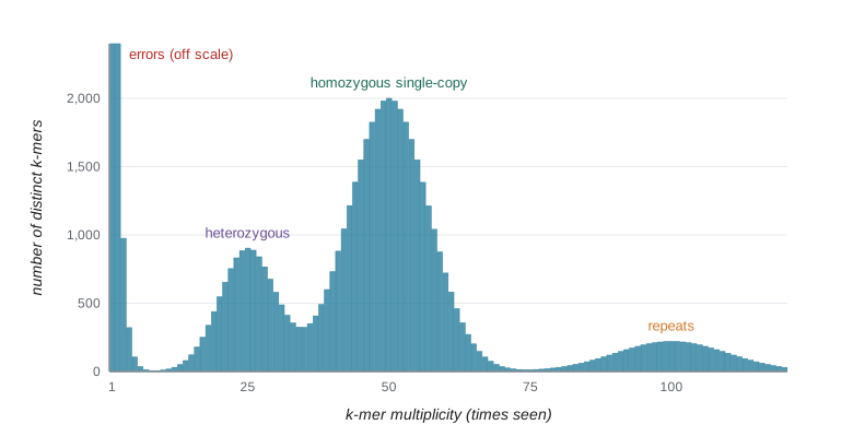
The spectrum yields a simple estimate of genome size. If the main peak lies at k-mer depth \(d\), and the total number of k-mers in the reads, excluding the error peak, is \(K\), then the genome size is approximately \(G \approx K/d\): each position in the genome is represented about \(d\) times. Tools such as GenomeScope fit a mixture model to the spectrum and estimate genome size, heterozygosity, repeat content and error rate together, all before assembly. This is invaluable for planning: a plant thought to have a 1 Gb genome that turns out to have a 3 Gb, highly heterozygous genome needs a very different sequencing budget.
# Estimate genome size from the k-mer spectrum of simulated reads with sequencing errors.
import random
from collections import Counter
random.seed(7)
G, L, cov, err, k = 60_000, 100, 25, 0.01, 21
genome = ''.join(random.choice('ACGT') for _ in range(G))
comp = str.maketrans('ACGT', 'TGCA')
def canonical(s):
    r = s.translate(comp)[::-1]
    return min(s, r)
counts = Counter()
n_reads = cov * G // L
for _ in range(n_reads):
    s = random.randrange(G - L + 1)
    read = list(genome[s:s + L])
    for i in range(L):
        if random.random() < err:
            read[i] = random.choice([b for b in 'ACGT' if b != read[i]])
    read = ''.join(read)
    if random.random() < 0.5:
        read = read.translate(comp)[::-1]
    for i in range(L - k + 1):
        counts[canonical(read[i:i + k])] += 1
spectrum = Counter(counts.values())
low_cut = 5
peak = max((m for m in spectrum if m >= low_cut), key=lambda m: spectrum[m])
solid = sum(m * n for m, n in spectrum.items() if m >= low_cut)
print('distinct k-mers seen once:', spectrum[1])
print('peak k-mer depth:', peak, ' expected about', round(cov * (L - k + 1) / L * (1 - err) ** k, 1))
print('estimated genome size:', round(solid / peak), ' true size:', G)distinct k-mers seen once: 218072 peak k-mer depth: 15 expected about 16.2 estimated genome size: 64763 true size: 60000
The peak lies where expected once errors are allowed for: read coverage of 25 becomes k-mer coverage of 20, and the roughly one in five 21-mers that contain an error are lost from the peak, leaving about 16. The size estimate is within about 8 percent of the truth; it runs slightly high because some error-containing k-mers recur often enough to pass the cut-off. Tens of thousands of distinct k-mers occur only once, almost all created by errors; counting tools discard them, and assemblers and error-correction programs use the same principle, treating k-mers well above the error threshold as solid and correcting read bases that create weak k-mers. Real k-mer counters such as Jellyfish and KMC handle billions of k-mers with efficient hashing and disk-based partitioning, and probabilistic structures such as Bloom filters store k-mer membership in a fraction of the memory.
Sketches and minimizers
Comparing whole read sets or genomes k-mer by k-mer is expensive, so many tools work with a sketch, a small random-like sample of k-mers chosen consistently. MinHash, the idea behind the Mash tool, keeps the \(s\) k-mers with the smallest hash values; the fraction shared between two sketches estimates the Jaccard similarity of the full k-mer sets, which in turn estimates the average nucleotide identity of two genomes. With sketches of a thousand k-mers, millions of bacterial genomes can be compared in minutes, which is how public databases are screened for close relatives of a new isolate. Minimizers, the smallest k-mer in each window of consecutive k-mers, give a related way to choose representative k-mers along a sequence; they underlie the minimap2 aligner (lesson 6) and many long-read assemblers.
| Step | Purpose | Typical tools | What can go wrong |
|---|---|---|---|
| Quality report | Spot instrument, library or contamination problems | FastQC, MultiQC | Misreading expected features (RNA-seq duplication) as failures |
| Adapter and quality trimming | Remove adapter read-through and poor bases | Cutadapt, fastp, Trimmomatic | Over-trimming bias; losing mate pairing |
| Contamination screen | Detect reads from other organisms | Kraken2, FastQ Screen | Database gaps cause false absence |
| k-mer counting and profiling | Estimate size, heterozygosity, repeats, errors | Jellyfish, KMC, GenomeScope | Wrong k or polyploidy misfits the model |
| Sketch comparison | Find close relatives, check identity | Mash, sourmash | Sketches too small for close comparisons |
Worked problem
Planning a genome project from a k-mer spectrum
An initial Illumina run on an invented wild grass gives 60 Gb of reads (150 bp). The 21-mer spectrum has an error peak, a peak at depth 18 and a taller peak at depth 36. The total number of k-mers outside the error peak is about 3.1 x 10^10. What can you infer?
Show solution
- Two peaks with one at half the depth of the other indicate a diploid (or diploid-like) genome with substantial heterozygosity; the peak at 36 is homozygous k-mers.
- Genome size is estimated as K divided by the homozygous peak depth: 3.1 x 10^10 / 36 ≈ 8.6 x 10^8, about 860 Mb.
- Read coverage is about 60 Gb / 0.86 Gb ≈ 70-fold; the k-mer depth of 36 is lower because each 150 bp read contains 130 21-mers and errors remove some.
- A tall heterozygous peak warns that a short-read assembly would fragment where haplotypes differ; long reads and a haplotype-aware assembler would be appropriate.
- Check the right-hand tail for repeat content before deciding how much long-read coverage to buy.
Answer: A heterozygous diploid genome of roughly 0.86 Gb; plan haplotype-resolved long-read assembly.
Common mistakes
MistakeTreating every FastQC warning as a failed sample.
InsteadInterpret metrics in context; high duplication is expected in RNA-seq, for example.
MistakeTrimming aggressively by default.
InsteadModern aligners soft-clip poor ends; heavy quality trimming can bias coverage and shorten useful reads.
MistakeAssuming coverage is Poisson in real data.
InsteadReal coverage is overdispersed by GC and mappability effects; plan for more depth than the model suggests.
MistakeConfusing k-mer depth with read depth.
Insteadk-mer depth is lower by the factor (L − k + 1)/L and further by errors.
MistakeChoosing a very small k for genome profiling.
InsteadWhen 4^k is not much larger than the genome size, k-mers repeat by chance and the spectrum blurs.
Summary and key terms
- Quality control reports are interpreted in the context of the experiment; MultiQC compares many samples at once.
- Adapter trimming remains essential; quality trimming by sliding window or the Mott maximum-segment method should be moderate.
- Coverage c = NL/G; under the Lander–Waterman Poisson model the uncovered fraction is e^−c, but real coverage is overdispersed.
- k-mers are substrings of length k; canonical k-mers merge a k-mer with its reverse complement.
- The k-mer spectrum reveals errors, heterozygosity, single-copy sequence and repeats, and estimates genome size as total k-mers divided by peak depth.
- MinHash sketches and minimizers summarize sequences for fast comparison and mapping.
- trimming
- Removing adapter sequence and low-quality bases from reads.
- coverage
- The number of reads overlapping a position, or its average over a genome.
- Lander–Waterman model
- A Poisson model of random read placement predicting coverage and gaps.
- k-mer
- A substring of length k.
- canonical k-mer
- The lexicographically smaller of a k-mer and its reverse complement.
- k-mer spectrum
- A histogram of how many distinct k-mers occur at each multiplicity.
- heterozygosity
- The proportion of sites at which the two haplotypes of a diploid differ.
- Bloom filter
- A probabilistic data structure that tests set membership compactly with some false positives.
- MinHash sketch
- A subset of k-mers with the smallest hash values, used to estimate set similarity.
- minimizer
- The smallest k-mer, by a chosen order, within a window of consecutive k-mers.
Practice problems
Work each problem on paper first, then reveal the answer to check.
A 5 Mb genome is sequenced with 2 million 150 bp reads. What is the mean coverage?
Show answer
2 x 10^6 x 150 / 5 x 10^6 = 60-fold.
At 3-fold coverage, what fraction of bases is expected to be uncovered under the Poisson model?
Show answer
e^−3 ≈ 0.05, about 5 percent.
How many 31-mers does a 150 bp read contain?
Show answer
120.
What is the canonical form of the 5-mer GGATC?
Show answer
Its reverse complement is GATCC; the smaller is GATCC.
Why does a diploid k-mer spectrum often show a peak at half the main depth?
Show answer
k-mers overlapping heterozygous sites occur on only one of the two haplotypes.
A spectrum peak lies at 40 and the solid k-mer total is 4.8 x 10^9. Estimate genome size.
Show answer
1.2 x 10^8, about 120 Mb.
Why are k-mers that occur once usually discarded?
Show answer
They are mostly created by sequencing errors.
What does MinHash estimate between two genomes?
Show answer
The Jaccard similarity of their k-mer sets, from which average nucleotide identity can be estimated.
Lesson quiz · 5 questions
Score 60% or more to complete this lesson.
Create a free account to save your progress, take quizzes and earn a certificate.