Genome annotation and hidden Markov models

An assembled genome is a long string of letters with no labels. Annotation adds the labels: where the genes are, how they are spliced, which proteins they encode, what those proteins probably do, and where repeats, noncoding RNAs and regulatory elements lie. Structural annotation locates features; functional annotation assigns them roles. Much of structural annotation rests on one of the most useful models in computational biology, the hidden Markov model, which this lesson develops in detail before turning to functional annotation, ontologies and the file formats that carry annotations.

Masking repeats

Annotation usually begins by identifying repeats, because transposable elements contain open reading frames of their own that would otherwise be mistaken for host genes, and because repeats cause spurious alignments. Tools such as RepeatMasker compare the genome with libraries of known repeat families, such as those in the Dfam database, and de novo tools such as RepeatModeler discover families specific to a new genome. The repeats are then masked: replaced by N (hard masking) or written in lower-case letters (soft masking), which lets later tools ignore them for seeding while still aligning across them. In many plant and animal genomes, more than half of the sequence is masked.

Finding genes in prokaryotes

Bacterial and archaeal genes are relatively easy to find. They are densely packed, mostly lack introns, and each is an open reading frame (ORF): a stretch from a start codon, usually ATG, to an in-frame stop codon (TAA, TAG or TGA). A random sequence contains a stop codon about every 21 codons on average (3 of the 64 codons), so ORFs of several hundred codons rarely arise by chance. But not every long ORF is a gene, especially in GC-rich genomes, where stop codons, being AT-rich, are rare in all frames. Programs such as Prodigal and GeneMarkS therefore score ORFs by codon usage and the composition of each codon position, typical of real genes in that genome, and look for a ribosome-binding site (Shine–Dalgarno sequence) upstream of the start codon. These programs predict bacterial genes with high accuracy, although the exact start codon is wrong more often than the gene itself.

# Find open reading frames on both strands of a synthetic sequence containing two planted genes.
import random
random.seed(8)
codons = [a + b + c for a in 'ACGT' for b in 'ACGT' for c in 'ACGT']
sense = [c for c in codons if c not in ('TAA', 'TAG', 'TGA')]
def gene(n_codons):
    return 'ATG' + ''.join(random.choice(sense) for _ in range(n_codons)) + 'TAA'
comp = str.maketrans('ACGT', 'TGCA')
rc = lambda s: s.translate(comp)[::-1]
filler = lambda n: ''.join(random.choice('ACGT') for _ in range(n))
seq = filler(300) + gene(150) + filler(250) + rc(gene(110)) + filler(200)
def orfs(s, min_codons=80):
    out = []
    for strand, t in (('+', s), ('-', rc(s))):
        for frame in range(3):
            i = frame
            while i + 3 <= len(t):
                if t[i:i + 3] == 'ATG':
                    for j in range(i, len(t) - 2, 3):
                        if t[j:j + 3] in ('TAA', 'TAG', 'TGA'):
                            if (j - i) // 3 >= min_codons:
                                start, end = (i + 1, j + 3) if strand == '+' else (len(s) - j - 2, len(s) - i)
                                out.append((strand, frame, start, end, (j - i) // 3))
                            i = j
                            break
                i += 3
    return out
print('sequence length', len(seq))
for strand, frame, start, end, n in sorted(orfs(seq), key=lambda r: r[2]):
    print(f"strand {strand} frame {frame}: {start}-{end} ({n} codons)")

sequence length 1542
strand + frame 0: 292-756 (154 codons)
strand - frame 2: 1007-1342 (111 codons)
strand + frame 2: 1128-1418 (96 codons)

The finder recovers both planted genes, on opposite strands. For the forward gene it reports a start nine bases upstream of the planted one, because an earlier in-frame ATG happens to occur with no stop codon in between; choosing among possible start codons is exactly where real gene finders use the ribosome-binding site. It also reports a third ORF of 96 codons on the forward strand, overlapping the reverse-strand gene: a shadow ORF on the opposite strand of a real gene, which arises because the reverse complement of coding sequence is depleted of stop codons. Composition-based gene finders recognize and reject such shadows.

Finding genes in eukaryotes

Eukaryotic gene prediction is much harder. Human protein-coding genes average about ten exons separated by introns that can be tens of thousands of bases long; coding sequence is a small fraction of the genome; alternative splicing produces several transcripts from most genes; and the signals marking exon boundaries are short and degenerate. Introns almost always begin with GT and end with AG, but those dinucleotides occur everywhere; the surrounding consensus sequences, the branch point and polypyrimidine tract add only a little information. Ab initio gene finders such as GENSCAN (1997) and AUGUSTUS combine many weak signals, splice-site scores, codon composition, exon and intron length distributions, into a probabilistic model of gene structure, a generalized hidden Markov model, and find the most probable parse of the sequence into exons, introns and intergenic regions.

Evidence greatly improves prediction. RNA-seq reads aligned with a splice-aware mapper (lesson 9) reveal exons and introns directly; long-read sequencing of full-length transcripts (Iso-Seq or direct RNA) reveals complete isoforms; and alignments of proteins from related species show conserved coding regions. Annotation pipelines such as BRAKER and MAKER train ab initio predictors on the evidence and combine everything into consensus gene models. The large reference annotations, Ensembl/GENCODE and NCBI RefSeq, add manual curation for important genomes. For clinical use, the two groups agreed the MANE (Matched Annotation from NCBI and EMBL-EBI) Select set, one representative transcript per human protein-coding gene that is identical in both annotations, so that variant descriptions are consistent across laboratories.

Noncoding RNA genes need their own methods. Transfer RNAs are found with tRNAscan-SE using their conserved cloverleaf structure, ribosomal RNAs by similarity to known rRNAs, and other families with covariance models in the Rfam database, which capture both sequence and secondary structure. Long noncoding RNAs, of which human annotations list tens of thousands, are identified from transcript evidence and lack of coding potential, and their functions are mostly unknown.

Hidden Markov models

A hidden Markov model (HMM) describes a sequence of observed symbols generated by an underlying sequence of hidden states. In a gene-finding HMM the observations are bases and the hidden states are labels such as exon, intron and intergenic; the states cannot be seen directly, but each state emits bases with its own characteristic probabilities. An HMM is defined by a set of states, transition probabilities \(a_{kl}\) between states, emission probabilities \(e_k(b)\) of symbol \(b\) in state \(k\), and initial probabilities. The model is Markov because the next state depends only on the current one.

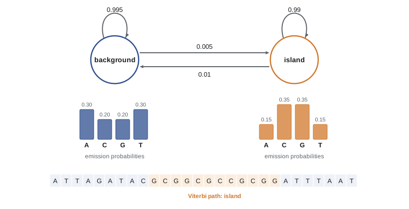
A classic teaching example, from the textbook by Richard Durbin and colleagues, is detecting CpG islands. In vertebrate genomes the dinucleotide CG is rare, because methylated cytosines in CG deamine to thymine and are lost over time, but in stretches of a few hundred to a few thousand bases, often at gene promoters, CG is unmethylated and remains common. A two-state HMM with states island and background, each emitting bases with different frequencies, can label a sequence. Three computational problems arise for any HMM: evaluating the probability of a sequence given the model (solved by the forward algorithm), finding the most probable path of hidden states (solved by the Viterbi algorithm) and estimating parameters from data (solved by the Baum–Welch algorithm, a form of expectation maximization, or by counting if labeled training data exist).

The Viterbi algorithm is dynamic programming again (lesson 5). Let \(v_k(i)\) be the probability of the most probable path that ends in state \(k\) after emitting the first \(i\) symbols. Then

and storing which \(k\) achieved the maximum allows the best path to be traced back. Because the products of many small probabilities underflow computer arithmetic, implementations work with logarithms, turning products into sums. The forward algorithm has the same structure with the maximum replaced by a sum, and gives the total probability of the sequence over all paths; combined with the analogous backward algorithm, it gives the posterior probability that each position is in each state, a measure of confidence in the labels.

# Simulate a sequence from a two-state CpG-island HMM and recover the islands with the Viterbi algorithm.
import math, random
random.seed(1)
states = ('B', 'I')                                   # background, island
trans = {'B': {'B': 0.995, 'I': 0.005}, 'I': {'B': 0.01, 'I': 0.99}}
emit = {'B': {'A': 0.30, 'C': 0.20, 'G': 0.20, 'T': 0.30},
        'I': {'A': 0.15, 'C': 0.35, 'G': 0.35, 'T': 0.15}}
def draw(d):
    r, acc = random.random(), 0
    for k, p in d.items():
        acc += p
        if r < acc:
            return k
    return k
path, seq, s = [], [], 'B'
for _ in range(3000):
    path.append(s); seq.append(draw(emit[s])); s = draw(trans[s])
lg = math.log
V = [{k: lg(0.5) + lg(emit[k][seq[0]]) for k in states}]
back = []
for x in seq[1:]:
    row, ptr = {}, {}
    for l in states:
        k_best = max(states, key=lambda k: V[-1][k] + lg(trans[k][l]))
        row[l] = V[-1][k_best] + lg(trans[k_best][l]) + lg(emit[l][x])
        ptr[l] = k_best
    V.append(row); back.append(ptr)
s = max(states, key=lambda k: V[-1][k])
decoded = [s]
for ptr in reversed(back):
    s = ptr[s]; decoded.append(s)
decoded.reverse()
def segments(p):
    out, start = [], None
    for i, st in enumerate(p + ['B']):
        if st == 'I' and start is None: start = i
        if st == 'B' and start is not None: out.append((start + 1, i)); start = None
    return out
agree = sum(a == b for a, b in zip(path, decoded)) / len(path)
print('true islands:   ', segments(path))
print('Viterbi islands:', segments(decoded))
print(f'positions decoded correctly: {agree:.1%}')

true islands:    [(474, 494), (725, 733), (739, 768), (938, 989), (1130, 1253), (1569, 1585), (1674, 1697), (1964, 2001), (2280, 2779)]
Viterbi islands: [(936, 994), (1096, 1253), (2279, 2778)]
positions decoded correctly: 93.9%

The Viterbi path recovers the three longest islands, with boundaries within a few bases to a few tens of bases of the truth, because a run of island-like composition at an edge is ambiguous. It misses the short islands of 9 to 50 bases: so few bases cannot outweigh the low probability of the two state switches needed to enter and leave the island state. About 94 percent of positions are labeled correctly. The posterior probabilities from the forward and backward algorithms would show how uncertain the boundaries and the short candidates are. Real gene finders use many more states, for exon phases, splice sites, start and stop codons and intron length classes, and generalized HMMs that model state durations explicitly, but the algorithms are the same.

Profile HMMs apply the same machinery to protein families. A profile HMM built from a multiple alignment has, for each column, a match state with position-specific emission probabilities, an insert state for extra residues and a delete state for skipped columns. Scoring a sequence against the model, with the forward algorithm, detects distant family members that pairwise BLAST would miss. HMMER, developed by Sean Eddy, searches sequences against the Pfam database of more than 20,000 protein families, and InterPro integrates Pfam with other family and domain databases.

Functional annotation and ontologies

Most predicted genes are assigned functions by homology: a predicted protein that is clearly homologous to a characterized protein, and that shares its domains and key residues, probably has a similar function. This inference is powerful but error-prone. Functions are often transferred from proteins that were themselves annotated by homology, so a single error can propagate through thousands of entries, and paralogues within a family can have different specificities. Annotations should therefore record their evidence.

The Gene Ontology (GO), started in 1998, provides a controlled vocabulary for describing gene function in three aspects: molecular function (such as protein kinase activity), biological process (such as response to DNA damage) and cellular component (such as mitochondrial inner membrane). Terms are organized in a directed acyclic graph from general to specific, and each annotation carries an evidence code: experimental evidence, such as a direct assay, is distinguished from inferences from sequence similarity and from electronic annotations made without curator review. Pathway databases such as KEGG and Reactome place genes in metabolic and signaling pathways. GO annotations underlie the enrichment analyses used to interpret lists of differentially expressed genes (lesson 9).

Annotation files and coordinates

Annotations are exchanged as GFF3 or GTF files, tab-separated lines giving sequence name, source, feature type (gene, mRNA, exon, CDS and so on), start, end, score, strand, frame and attributes linking features, such as ID and Parent. GFF and GTF use 1-based, fully closed coordinates: a feature from 101 to 200 includes both ends and is 100 bases long. BED files, used for intervals in genome browsers and many tools, use 0-based, half-open coordinates: the same feature is written 100 to 200. Confusing the two systems is one of the commonest errors in bioinformatics, producing off-by-one errors that shift every feature by a base.

# Parse an invented GFF3 gene model, compute exon, intron and CDS lengths, and convert exons to BED.
gff = """chr3\tdemo\tgene\t1001\t5200\t.\t+\t.\tID=gene1;Name=XYZ1
chr3\tdemo\tmRNA\t1001\t5200\t.\t+\t.\tID=tx1;Parent=gene1
chr3\tdemo\texon\t1001\t1300\t.\t+\t.\tParent=tx1
chr3\tdemo\texon\t2101\t2350\t.\t+\t.\tParent=tx1
chr3\tdemo\texon\t4801\t5200\t.\t+\t.\tParent=tx1
chr3\tdemo\tCDS\t1151\t1300\t.\t+\t0\tParent=tx1
chr3\tdemo\tCDS\t2101\t2350\t.\t+\t0\tParent=tx1
chr3\tdemo\tCDS\t4801\t5051\t.\t+\t2\tParent=tx1"""
exons, cds = [], []
for line in gff.splitlines():
    f = line.split('\t')
    start, end = int(f[3]), int(f[4])
    if f[2] == 'exon': exons.append((start, end))
    if f[2] == 'CDS': cds.append((start, end))
length = lambda iv: iv[1] - iv[0] + 1                        # GFF: 1-based, closed
introns = [(a[1] + 1, b[0] - 1) for a, b in zip(exons, exons[1:])]
cds_len = sum(map(length, cds))
print('exon lengths:', [length(e) for e in exons], ' mature transcript:', sum(map(length, exons)), 'nt')
print('intron lengths:', [length(i) for i in introns])
print('CDS length:', cds_len, 'nt =', cds_len // 3, 'codons; divisible by 3:', cds_len % 3 == 0)
print('BED lines (0-based, half-open):')
for s, e in exons:
    print(f"chr3\t{s - 1}\t{e}")

exon lengths: [300, 250, 400]  mature transcript: 950 nt
intron lengths: [800, 2450]
CDS length: 651 nt = 217 codons; divisible by 3: True
BED lines (0-based, half-open):
chr3	1000	1300
chr3	2100	2350
chr3	4800	5200