
BAS-130 · Lesson 6 of 12 · 26 min
Tuning a PID loop
▶ Video coming soon A video version of this lesson is on the way.
On Friday, October 16, Callie arrived at the Tilden basement at 7:30, an hour earlier than usual, because Prakash wanted the hot water converter at a steady, moderate load for a step test before the building filled up. Nell Nakagawa had agreed to the test the week before and had asked them to keep the water within a few degrees of setpoint and to stop at once if the steam pressure did anything strange. Prakash put the converter loop into manual, held the steam valve where it was for five minutes to let everything settle, and then moved it by a known amount. For the next ten minutes Callie watched the water temperature respond and wrote down what she saw. "Everything you need to tune this loop is in the next ten minutes," he said. "How long it takes to start moving, how fast it moves and how far it goes."
Tuning means choosing a loop's gain, integral time and, rarely, derivative time so that it holds setpoint and recovers from upsets quickly without overshooting much or hunting. Lessons 4 and 5 explained what each action does. This lesson covers how to choose the numbers: the safety and courtesy that come first, a practical manual method, the step test and the simple rules that turn its results into settings, and how to check and record the result.
Before you touch a loop
Tuning means changing how a building system behaves, often on equipment that serves occupied spaces or feeds other systems. A few habits keep it safe. Talk to the building operator first, explain what you will do and agree when. Pick a time when the load is steady and representative, not during morning start-up or when a lab is running an experiment. Record every setting before you change it. Know the safe limits of the process, such as the highest and lowest acceptable water or air temperatures, and stay well inside them. And never tune a loop whose safeties are bypassed or whose equipment has a known fault, because a loop that looks badly tuned is often a loop with a mechanical problem.
That last point matters more than any tuning rule. Before tuning, Prakash always checked that the sensor read correctly, that the actuator stroked fully and followed its command, and that nothing was obviously sticking or slipping. On the converter he had stroked the steam valve the previous afternoon and found it smooth. On a VAV box in Ninefield the week before, a hunting loop had turned out to be a cracked flow pickup tube, which no setting could have fixed.
A practical manual method
Many experienced technicians tune most building loops by hand, using a method something like this. Start with integral action slow and derivative off. Raise the gain in steps, making a small setpoint change after each step and watching the response, until the process variable just begins to overshoot and swing before settling. Back the gain off to roughly half that value. Then speed up integral action, shortening the integral time, until the offset disappears at a reasonable rate without the loop starting to swing slowly. Finally make a setpoint change and, if possible, a load change, and confirm that the loop recovers well from both.
The method works because it finds the edge of stability and then steps back to a safe margin. Its drawback is time: each step needs the loop to settle, which can take minutes on a fast loop and hours on a slow one. For slow loops such as room temperatures, or for a loop that has to be right the first time, a step test gives starting values more quickly.
The step test
A step test, also called a bump test or open-loop test, measures how the process responds to a change in output with the loop out of the way. With the loop in manual and the process steady, the output is stepped by a known amount, typically 5 to 15 in 100 of its range, and the process variable is recorded until it settles at its new value. Three numbers describe the response well enough for tuning. The process gain is how much the process variable changed divided by how much the output changed. The dead time is the delay between the output step and the first visible movement of the process variable. The time constant is how long the process variable then takes to complete about 63 in 100 of its total change.
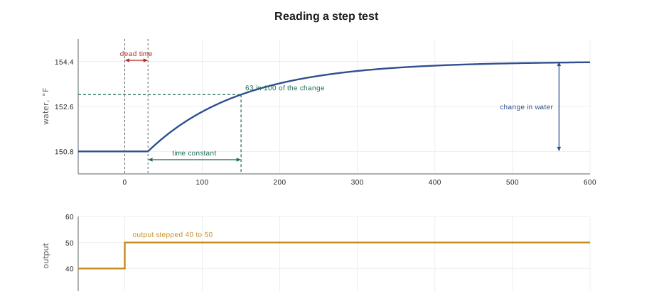
The 63 in 100 figure comes from the shape of a simple first-order response, which rises by about 63 in 100 of its final change in one time constant, 86 in 100 in two and 95 in 100 in three. Real building processes are not perfectly first order, but most air and water temperature loops are close enough for the numbers to give good starting settings.
Worked problem
Reading the converter step test
With the converter loop in manual, Prakash stepped the steam valve from 40 to 50 in 100. The hot water supply had been steady at 150.8 °F. Nothing happened for about 30 seconds; the water then rose and settled at 154.4 °F. It reached 153.1 °F, about 63 in 100 of the way, 150 seconds after the step. Find the process gain, dead time and time constant.
Show solution
- Change in output: 50 − 40 = 10.
- Change in temperature: 154.4 − 150.8 = 3.6 °F.
- Process gain: 3.6 ÷ 10 = 0.36 °F per unit of output.
- 63 in 100 point: 150.8 + 0.632 × 3.6 = 153.1 °F, reached at 150 s.
- Dead time: 30 s. Time constant: 150 − 30 = 120 s.
Answer: Process gain 0.36 °F per unit, dead time 30 seconds, time constant 120 seconds.
Callie noticed one more thing: the ratio of dead time to time constant, here 30 to 120, or 0.25. Prakash called it the difficulty number. A loop whose dead time is small compared with its time constant is easy to control tightly. As dead time grows toward the time constant, the loop must be tuned more gently, because the controller is always acting on old information. Lesson 10 returns to dead time as a cause of hunting.
From step test to settings: the lambda method
Several sets of rules turn step test results into PI settings. One that suits building loops well is the lambda method, also called internal model control tuning. The technician chooses how quickly the loop should respond after a change, a target called lambda, as a time. A lambda equal to the process time constant gives a calm, robust loop that does not overshoot; a smaller lambda gives a faster but less forgiving loop. The integral time is set equal to the process time constant, and the gain follows from a simple formula.
Here τ is the time constant, θ the dead time, K the process gain and λ the chosen response time. The formula gives the gain in the same units the controller uses, output per unit of process variable, when K is in process variable units per unit of output.
Worked problem
Lambda settings for the converter
Using the step test results, with lambda set equal to the time constant, find the gain, throttling range and integral time for the converter.
Show solution
- λ = τ = 120 s; θ = 30 s; K = 0.36 °F per unit.
- Kc = 120 ÷ (0.36 × (120 + 30)) = 120 ÷ 54 = 2.22 per °F.
- Throttling range: 100 ÷ 2.22 = 45 °F.
- Integral time: Ti = τ = 120 s, or 2 minutes.
Answer: A gain of 2.22 per °F, a throttling range of 45 °F and an integral time of 2 minutes, a gentler gain and faster integral than the 6.94 per °F and 5 minutes the loop had been running with.
The throttling range of 45 °F surprised Callie, after lesson 4's warning about wide throttling ranges and offset. Prakash explained that with integral action doing the work of removing offset, the gain only has to provide a firm, stable first response. A wide throttling range is no problem in a PI loop; it is only a problem when proportional action has to work alone.
Ziegler–Nichols and why to be careful with it
The best-known tuning rules are those published by Ziegler and Nichols in the 1940s. Their open-loop rules use the same three step-test numbers. For a PI controller they give a gain of 0.9 times the time constant divided by the product of process gain and dead time, and an integral time of about 3.3 times the dead time. Their closed-loop method raises the gain of a P-only loop until it swings steadily and uses that gain and the period of the swing.
Worked problem
Ziegler–Nichols PI settings for comparison
Using the same step test, what PI settings do the Ziegler–Nichols open-loop rules give?
Show solution
- Kc = 0.9 × 120 ÷ (0.36 × 30) = 108 ÷ 10.8 = 10 per °F.
- Ti = 3.33 × 30 = about 100 s.
Answer: A gain of 10 per °F, more than four times the lambda value, with a similar integral time.
Ziegler and Nichols aimed for a response that overshoots and then dies out with each swing about a quarter the size of the one before. That is quick, but it is too lively for most building systems, where overshoot wastes energy, upsets occupants and wears valves, and where conditions change through the day and the season. Many technicians use Ziegler–Nichols settings, if at all, only as an upper limit and then reduce the gain. The closed-loop method also needs the loop deliberately driven into steady oscillation, which is rarely acceptable in an occupied building.
Checking the result
Settings from any rule are starting values. After entering them, put the loop back in automatic and test it two ways. A setpoint step, such as lowering the setpoint by a degree, shows how the loop tracks a change. A load disturbance, such as a fan start, another valve opening or simply the normal morning load rise, shows how it rejects an upset, which is what most building loops spend their lives doing. A good result settles in a few time constants with little overshoot. If it is sluggish, raise the gain a little or shorten the integral time a little; if it swings, do the opposite. Change one setting at a time.
On the converter, Prakash entered the lambda settings at 8:10 and lowered the setpoint by 2 degrees for a test. The water fell smoothly to the new setpoint in about seven minutes with almost no overshoot. When AHU-1's heating coil opened at 8:25 and drew more heat, the water dipped by about half a degree and recovered in five minutes. That was gentler than the old settings, which had overshot by more than a degree on every morning start. Nell watched the trend for a week before agreeing to keep the new values.
Typical loop speeds
Building loops differ enormously in speed, and their settings differ with them. A duct static pressure loop responds within seconds; a room temperature loop may take half an hour. The table gives typical ranges as a guide to whether settings are in a sensible region. They are not rules: every installation differs, and the step test or manual method decides.
| Loop | Typical dead time | Typical time constant | Typical integral time |
|---|---|---|---|
| Duct or building static pressure | About a second | A few seconds | 10 to 60 s |
| Water differential pressure on pumps | A few seconds | Several seconds | 20 to 90 s |
| Supply or discharge air temperature | 10 to 60 s | 1 to 3 minutes | 1 to 3 minutes |
| Hot water or chilled water supply temperature | 20 to 90 s | 1 to 5 minutes | 2 to 5 minutes |
| Mixed air temperature on dampers | 5 to 30 s | 30 s to 2 minutes | 30 s to 2 minutes |
| Room or zone temperature | Several minutes | 10 to 30 minutes or more | 10 to 30 minutes |
Auto-tuning and its limits
Many controllers offer an auto-tune function that bumps the output, watches the response and calculates settings itself. Some run continuously and adapt as conditions change. Auto-tuning is convenient and often gives sound results, but it is only as good as the conditions during the test. A tune run while a mechanical fault is present, while another loop is swinging or at a load far from normal gives settings that suit those conditions. Treat auto-tuned values like any other starting point: check the response and record the result.
Two other cautions apply to every method. Building processes are nonlinear: a hot water coil gives most of its heat in the first part of its valve travel, and a fan's pressure rises with the square of its speed, so a loop tuned at one load may be too lively or too sluggish at another. Tune at a representative load and check at the extremes if you can. And loops interact: an air handler's static pressure loop and its VAV box flow loops affect each other, as do a mixed air loop and a supply air loop. Tune the inner, faster loops first and the outer, slower loops last, one at a time.
Recording the work
Every tuning job ends with a record: the loop's name, the date, the old and new settings, the conditions during the test, and the response seen. Quillon kept these on the job's commissioning sheet and in a comment field in the controller program itself, so that the next technician would know who had changed what and why. Prakash had found too many loops over the years with settings nobody could explain. "If you can't say why a number is what it is, you're one bad Monday from someone changing it back," he said.
Common mistakes
MistakeTuning a loop before checking the sensor, actuator and valve.
InsteadRule out mechanical faults first; many badly behaved loops are not tuning problems.
MistakeRunning a step test during morning start-up or a changing load.
InsteadTest at a steady, representative load so the response reflects the process.
MistakeUsing Ziegler–Nichols settings as final values in an occupied building.
InsteadTreat them as an upper limit; building loops usually need gentler gains.
MistakeChanging gain and integral time at the same time.
InsteadChange one setting, test, then change the next.
MistakeTuning outer loops before inner loops.
InsteadTune the faster inner loops first, then the slower outer loops.
MistakeLeaving no record of new settings.
InsteadRecord old and new values, the date, the conditions and the result.
Summary and key terms
- Tuning chooses gain and integral time so a loop holds setpoint and recovers from upsets without much overshoot or hunting.
- Talk to the operator, pick a steady load, record settings and rule out mechanical faults before tuning.
- Manual tuning raises gain until the loop just swings, backs it off, then speeds up integral until offset clears.
- A step test measures process gain, dead time and time constant (the time to about 63 in 100 of the change).
- The lambda method sets the integral time equal to the time constant and calculates a gain from the chosen response time.
- Ziegler–Nichols rules give lively settings that are usually too aggressive for buildings.
- Check settings with a setpoint step and a load change, change one setting at a time, and record the result.
- Tuning
- Choosing a loop's gain, integral and derivative settings.
- Step test
- A test in which the output is stepped in manual and the process response is recorded; also called a bump test.
- Process gain
- The change in process variable divided by the change in output that caused it.
- Dead time
- The delay between a change in output and the first visible response of the process variable.
- Time constant
- The time a first-order process takes to complete about 63 in 100 of its response after the dead time.
- Lambda tuning
- A tuning method in which the technician chooses the loop's response time and calculates settings from a step test.
- Auto-tune
- A controller function that tests the process and calculates its own settings.
Practice problems
Work each problem on paper first, then reveal the answer to check.
A step of 10 in 100 raises a supply air temperature by 5.4 °F. What is the process gain?
Show answer
5.4 ÷ 10 = 0.54 °F per unit of output.
After a step, a process starts moving at 15 seconds and reaches 63 in 100 of its change at 75 seconds. What are its dead time and time constant?
Show answer
Dead time 15 s; time constant 75 − 15 = 60 s.
Using the lambda method with λ = τ = 60 s, θ = 15 s and K = 0.54 °F per unit, what is the gain?
Show answer
60 ÷ (0.54 × 75) = 1.48 per °F, with an integral time of 60 s.
Why tune inner loops before outer loops?
Show answer
The outer loop's behavior depends on the inner loop; tuning it first wastes the work when the inner loop changes.
What should you do before running a step test on a plant loop?
Show answer
Agree the test with the operator, choose a steady load, record the settings and know the safe limits.
Lesson quiz · 5 questions
Score 60% or more to complete this lesson.
Create a free account to save your progress, take quizzes and earn a certificate.