Formulating problems: rewards, horizons and partial observability

Dynamic programming (Lesson 3) solves a Markov decision process once it is written down. In practice, writing it down is often the hardest part. What counts as the state? What reward will produce the behavior we actually want? Should future rewards be discounted, and by how much? What if the agent cannot observe the state at all? A poorly formulated problem can be solved perfectly and still produce useless or harmful behavior. This lesson covers the design of states and actions, reward design and shaping, reward hacking, discounting and average reward, episodic and continuing tasks, constraints, and partially observable MDPs, in which the agent must act on beliefs rather than states.

Choosing states and actions

The Markov property (Lesson 1) requires the state to summarize everything about the past that matters for the future. Whether a formulation is Markov depends on what is included:

• A single camera image of a moving ball is not Markov, because it shows position but not velocity; stacking several recent frames, as DQN does for Atari games (Lesson 7), restores much of the missing information.
• For a thermostat, room temperature alone is not Markov if the heating system has thermal lag; adding the temperature trend or the heater's recent output helps.
• For inventory control, the stock level plus outstanding orders and the day of the week may suffice.

Including more variables makes the state more nearly Markov but enlarges the state space, the curse of dimensionality of Lesson 3. Good state design keeps what is predictive and drops what is not, often using domain knowledge.

Actions also need care. Their granularity sets the time scale of decisions: a robot controlled by joint torques at 1 kHz faces a very long horizon, while one choosing among pre-programmed skills (reach, grasp, place) faces a short one. Hierarchical formulations, such as options (temporally extended actions with their own policies and termination conditions), let agents plan at several time scales. Continuous actions require different algorithms from discrete ones (Lesson 9), and large discrete action sets, such as choosing among millions of items to recommend, need embedding or candidate-generation approaches.

Designing rewards

The reward hypothesis holds that any goal can be expressed as maximizing expected cumulative reward. In principle this is true; in practice, choosing a reward that leads to the intended behavior is difficult. Two broad styles exist:

• Sparse rewards describe only the outcome: +1 for winning a game, reaching a goal or completing a task, 0 otherwise. They are easy to specify correctly but hard to learn from, because the agent may wander for a very long time before ever receiving a signal.
• Dense (shaped) rewards add intermediate signals, such as progress toward a goal or penalties for energy use. They speed learning but risk rewarding the wrong thing.

The guiding principle is to reward what you want achieved, not how you think it should be achieved. Rewarding a chess agent for capturing pieces would produce an agent that captures greedily rather than one that wins.

Reward shaping without changing the optimal policy

Ng, Harada and Russell (1999) showed that adding a shaping reward of the form

for any function \(\Phi\) of the state, called a potential, leaves the optimal policy unchanged. Along any trajectory, the shaping terms telescope: their discounted sum equals \(-\Phi(s_0)\) plus a vanishing term, which does not depend on the actions taken. A good potential, such as an estimate of distance to the goal or an approximate value function, gives the agent immediate feedback for progress without creating new optimal behavior. Shaping rewards not of this form can change the optimal policy in unexpected ways.

import numpy as np

# Corridor of 6 states; the goal (state 5) gives +10 and ends the episode. Each step costs nothing else. gamma = 0.9
n, gamma = 6, 0.9
def value_iteration(bonus):
    """bonus(s, s2): extra reward added to every transition; returns the greedy policy."""
    V = np.zeros(n)
    for _ in range(500):
        newV = V.copy()
        for s in range(n - 1):
            qs = []
            for s2 in (max(s - 1, 0), s + 1):          # actions: left, right
                r = (10 if s2 == n - 1 else 0) + bonus(s, s2)
                qs.append(r + gamma * (0 if s2 == n - 1 else V[s2]))
            newV[s] = max(qs)
        V = newV
    policy = []
    for s in range(n - 1):
        qs = [(10 if s2 == n - 1 else 0) + bonus(s, s2) + gamma * (0 if s2 == n - 1 else V[s2]) for s2 in (max(s - 1, 0), s + 1)]
        policy.append("L" if qs[0] > qs[1] else "R")
    return "".join(policy)

print("no shaping:               ", value_iteration(lambda s, s2: 0.0))
# Naive shaping: +3 for being in state 2 (a "checkpoint"). The agent learns to bounce around it.
print("naive bonus for state 2:  ", value_iteration(lambda s, s2: 3.0 if s2 == 2 else 0.0))
# Potential-based shaping F = gamma * phi(s2) - phi(s), with phi = progress toward the goal
phi = np.arange(n) * 2.0
print("potential-based shaping:  ", value_iteration(lambda s, s2: gamma * (0 if s2 == n - 1 else phi[s2]) - phi[s]))

no shaping:                RRRRR
naive bonus for state 2:   RRRLL
potential-based shaping:   RRRRR

With a naive bonus of +3 for entering state 2, the agent in states 3 and 4 turns back to collect the bonus repeatedly instead of finishing, because looping earns more than the goal. Potential-based shaping, rewarding progress through \(\Phi(s) = 2s\), keeps the original optimal policy.

Reward hacking

Agents optimize the reward they are given, not the one intended, and will exploit any gap between the two. Documented examples include a boat-racing agent that circled endlessly collecting respawning targets instead of finishing the race, simulated robots that exploited physics-engine bugs to move by vibrating, and agents that learned to pause a game forever to avoid losing. In language models trained with learned reward models (Lesson 12), the policy can learn to produce outputs the reward model scores highly but humans do not prefer, such as longer or more flattering answers. This is an instance of Goodhart's law: when a measure becomes a target, it ceases to be a good measure.

Defenses include: keeping rewards close to true outcomes; testing learned behavior adversarially; constraining how far the policy can move from a trusted reference (such as the KL penalty in RLHF, Lesson 12); using several reward signals that are hard to satisfy simultaneously by exploitation; and, for important deployments, human review of what the agent actually does.

Horizons and discounting

Tasks are either episodic, ending in terminal states (a game, a delivery, a conversation), or continuing, running indefinitely (process control, a recommender serving users forever). For continuing tasks the undiscounted sum of rewards may be infinite, so a discount factor \(\gamma < 1\) or an average reward criterion is needed.

The discount factor has several interpretations: a modeling convenience that keeps returns finite; a preference for sooner rewards; a probability \(1 - \gamma\) that the process ends at each step; and a way to set an effective horizon of about \(1/(1 - \gamma)\) steps, beyond which rewards barely matter. With \(\gamma = 0.99\) the horizon is about 100 steps; with 0.999, about 1,000.

Larger discount factors make learning harder: returns have higher variance, and errors in value estimates propagate over longer chains. Practical algorithms often use a somewhat smaller \(\gamma\) than the true problem would suggest, trading bias for stability.

For continuing tasks the average reward criterion, \(r(\pi) = \lim_{T \to \infty}\frac1T\mathbb{E}\left[\sum_{t=1}^{T} R_t\right]\), avoids discounting altogether. Values are then defined relative to the average (differential values), and there are average-reward versions of the TD methods of Lesson 5. It suits problems such as queueing control and data center cooling, where the long-run rate of reward is what matters.

Constraints and safety

Many real objectives have constraints: keep temperature within limits, keep the probability of collision below a threshold, stay within a budget. Folding constraints into the reward as penalties requires choosing the penalty weights, and the agent may still trade a constraint violation for enough reward. Constrained MDPs make the trade-off explicit: maximize expected return subject to expected costs staying below limits. A standard solution introduces Lagrange multipliers, one per constraint, and alternates between improving the policy for the penalized reward and increasing the multiplier when the constraint is violated or decreasing it when the constraint is satisfied with slack. Safe exploration, ensuring that the agent never takes catastrophic actions while learning, usually requires additional structure such as shields that block unsafe actions, conservative policies derived from offline data (Lesson 10), or training in simulation.

Partially observable MDPs

In many problems the agent cannot see the state: a robot's sensors are noisy, a dialogue system cannot read the user's intent, a maintenance planner cannot observe hidden wear. A partially observable MDP (POMDP) adds an observation model \(O(o \mid s', a)\) giving the probability of each observation after an action. The agent must act on the history of observations, which can be summarized without loss by the belief state, the posterior distribution over states:

This is the Bayes filter of AI-320 (Lesson 11): predict with the transition model, then weight by the observation likelihood. The belief is a sufficient statistic, and the POMDP becomes an MDP over beliefs, with continuous state even if the original states are discrete. Optimal policies trade off information gathering against reward: it can be worth taking an action with no immediate benefit because it reduces uncertainty.

The classic illustration is the tiger problem: a tiger is behind one of two doors, the agent can listen (costing 1, and correct 85% of the time) or open a door (+10 for the safe door, −100 for the tiger).

import numpy as np

# The tiger problem: a tiger is behind the left or right door. Listening costs 1 and hears the
# correct side with probability 0.85. Opening the tiger door costs 100; the other door pays +10.
def update(b, heard_left, acc=0.85):
    """Bayes update of the belief that the tiger is on the left."""
    like_left = acc if heard_left else 1 - acc
    like_right = 1 - acc if heard_left else acc
    return like_left * b / (like_left * b + like_right * (1 - b))

def open_value(b):
    # best expected reward from opening a door now: open right if tiger likely left, and vice versa
    return max(b * 10 + (1 - b) * -100, (1 - b) * 10 + b * -100)

b = 0.5
for obs in ["left", "left", "right", "left"]:
    b = update(b, obs == "left")
    print(f"heard {obs:5s}: P(tiger left) = {b:.3f}; expected reward of opening now = {open_value(b):+.1f}")

# A simple policy: listen until the belief passes a threshold, then open. Simulate its average return.
rng = np.random.default_rng(3)
for thr in (0.85, 0.97, 0.995):
    total = 0.0
    for _ in range(20000):
        tiger_left = rng.random() < 0.5; b = 0.5; ret = 0.0
        while max(b, 1 - b) < thr:
            heard_left = (rng.random() < 0.85) == tiger_left
            b = update(b, heard_left); ret -= 1
        open_right = b > 0.5
        ret += 10 if open_right == tiger_left else -100
        total += ret
    print(f"open when confidence reaches {thr}: average return {total / 20000:+.2f}")

heard left : P(tiger left) = 0.850; expected reward of opening now = -6.5
heard left : P(tiger left) = 0.970; expected reward of opening now = +6.7
heard right: P(tiger left) = 0.850; expected reward of opening now = -6.5
heard left : P(tiger left) = 0.970; expected reward of opening now = +6.7
open when confidence reaches 0.85: average return -7.74
open when confidence reaches 0.97: average return +5.18
open when confidence reaches 0.995: average return +4.21

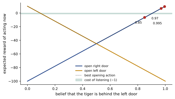
One "heard left" observation raises the belief to 0.85, which is not enough: opening the right door would still have an expected reward of −6.5. Two consistent observations give 0.97 and a positive expected reward. Waiting for 0.995 costs an extra listen for little gain. The best threshold balances the cost of information against the risk of a catastrophic choice, the essence of decision-making under partial observability.

Exact POMDP solutions are intractable beyond small problems, but practical methods include point-based value iteration, online planning from the current belief with Monte Carlo tree search (Lesson 6), particle filters for belief tracking, and, in deep RL, recurrent networks or transformers that learn an internal representation of history. Treating the most recent observation as if it were the state, a common shortcut, works when observations are nearly Markov and fails when important information is hidden.