Dynamic programming

When the MDP is known, meaning the transition probabilities and rewards are available, optimal policies can be computed rather than learned. Dynamic programming (DP), developed by Richard Bellman in the 1950s, solves the Bellman equations by turning them into update rules and iterating. DP is rarely applied directly to large problems, because it needs a complete model and sweeps over every state, but it is the conceptual foundation of all of RL: Monte Carlo, temporal-difference, Q-learning and actor-critic methods can all be understood as ways of approximating DP without a model and without visiting every state. This lesson covers policy evaluation, policy improvement, policy iteration and value iteration, their convergence, generalized policy iteration, and the curse of dimensionality.

Policy evaluation

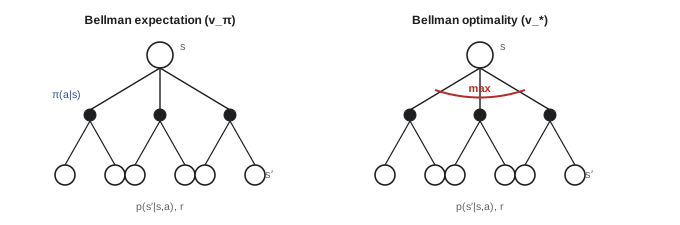
Policy evaluation computes \(v_\pi\) for a given policy. For small problems the Bellman equations can be solved directly as a linear system, as in Lesson 1, but that costs \(O(|\mathcal S|^3)\). Iterative policy evaluation instead turns the Bellman equation into an update applied to every state in a sweep:

Starting from any \(v_0\), for example all zeros, the sequence converges to \(v_\pi\) as \(k \to \infty\). The reason is that the Bellman operator \(T_\pi\), which maps a value function to the right-hand side, is a \(\gamma\)-contraction in the maximum norm: \(\|T_\pi v - T_\pi u\|_\infty \le \gamma\|v - u\|_\infty\). Each sweep shrinks the error by at least a factor of \(\gamma\), so the error after \(k\) sweeps is at most \(\gamma^k\) times the initial error. In practice, sweeps stop when the largest change in any state falls below a small threshold.

Each update replaces the estimate of a state's value with an expectation over successor states using their current estimates. This idea, updating estimates on the basis of other estimates, is called bootstrapping, and it is central to most RL methods. Updating in place, using new values as soon as they are computed within a sweep (like Gauss-Seidel in ELE-380), usually converges faster than keeping two arrays.

Policy improvement

Knowing \(v_\pi\), can we find a better policy? Compute the action values \(q_\pi(s, a) = \sum_{s'} p(s' \mid s, a)[r(s, a) + \gamma v_\pi(s')]\) and act greedily:

The policy improvement theorem guarantees that \(\pi'\) is at least as good as \(\pi\) in every state: \(v_{\pi'}(s) \ge v_\pi(s)\). Intuitively, choosing a better action in one state and then following \(\pi\) is better than following \(\pi\) throughout, and repeating the argument at every step shows that following \(\pi'\) throughout is better still. If the greedy policy is no better than \(\pi\) anywhere, then \(v_\pi\) satisfies the Bellman optimality equation and \(\pi\) is optimal.

Policy iteration

Policy iteration alternates the two steps: evaluate the current policy, improve it greedily, and repeat until the policy stops changing. Because a finite MDP has a finite number of deterministic policies and each iteration produces a strictly better policy until the optimum, policy iteration converges in a finite number of iterations, usually very few, even for large state spaces.

import numpy as np

P = {0: np.array([[0.8, 0.2, 0.0], [0.0, 0.7, 0.3], [0.0, 0.0, 1.0]]),
     1: np.array([[1.0, 0.0, 0.0], [1.0, 0.0, 0.0], [1.0, 0.0, 0.0]])}
R = {0: np.array([10.0, 6.0, 0.0]), 1: np.array([-4.0, -4.0, -12.0])}
gamma, names = 0.95, ["run", "repair"]

def q_values(V):
    return np.array([R[a] + gamma * P[a] @ V for a in (0, 1)])     # shape (actions, states)

# policy iteration: evaluate exactly, then improve greedily
policy = np.array([0, 0, 0])                                         # start: never repair
for it in range(1, 10):
    P_pi = np.array([P[policy[s]][s] for s in range(3)])
    R_pi = np.array([R[policy[s]][s] for s in range(3)])
    V = np.linalg.solve(np.eye(3) - gamma * P_pi, R_pi)
    new = q_values(V).argmax(axis=0)
    print(f"PI iteration {it}: policy {[names[a] for a in policy]}  V = {np.round(V, 2)}")
    if np.array_equal(new, policy):
        break
    policy = new

# value iteration on the same MDP
V = np.zeros(3)
for k in range(1, 1000):
    V_new = q_values(V).max(axis=0)
    if np.max(np.abs(V_new - V)) < 1e-6:
        break
    V = V_new
print(f"value iteration: {k} sweeps to converge, V = {np.round(V, 2)}, policy {[names[a] for a in q_values(V).argmax(axis=0)]}")

PI iteration 1: policy ['run', 'run', 'run']  V = [55.85 17.91  0.  ]
PI iteration 2: policy ['run', 'repair', 'repair']  V = [155.29 143.53 135.53]
value iteration: 310 sweeps to converge, V = [155.29 143.53 135.53], policy ['run', 'repair', 'repair']

Starting from "never repair", one round of evaluation and improvement finds the optimal policy, "run when good, repair when worn or broken", and the second evaluation confirms that it no longer changes. Value iteration, described next, reaches the same values but needs hundreds of cheap sweeps, because with \(\gamma = 0.95\) the error shrinks by only 5% per sweep.

Value iteration

Policy iteration evaluates each policy fully, which can be wasteful when the policy will soon change anyway. Value iteration combines a single sweep of evaluation with improvement, by applying the Bellman optimality equation as an update:

The Bellman optimality operator is also a \(\gamma\)-contraction, so value iteration converges to \(v_*\) from any start. When the values have converged to within a tolerance, the greedy policy with respect to them is optimal or near-optimal; in fact the greedy policy often becomes optimal long before the values have converged.

import numpy as np

# 4 x 5 gridworld: G goal (+10, terminal), X pit (-10, terminal), # wall, step reward -1.
grid = ["....G",
        ".#..X",
        ".....",
        "S...."]
H, W = len(grid), len(grid[0])
moves = {"^": (-1, 0), "v": (1, 0), "<": (0, -1), ">": (0, 1)}
perp = {"^": "<>", "v": "<>", "<": "^v", ">": "^v"}
gamma, slip = 0.95, 0.2                       # intended move with prob 0.8, each perpendicular 0.1

def step(r, c, a):
    dr, dc = moves[a]
    r2, c2 = r + dr, c + dc
    if not (0 <= r2 < H and 0 <= c2 < W) or grid[r2][c2] == "#":
        return r, c
    return r2, c2

def outcomes(r, c, a):
    res = [(1 - slip, step(r, c, a))]
    res += [(slip / 2, step(r, c, b)) for b in perp[a]]
    return res

V = np.zeros((H, W)); sweeps = 0
while True:
    delta = 0.0
    for r in range(H):
        for c in range(W):
            if grid[r][c] in "GX#":
                continue
            best = -1e9
            for a in moves:
                q = 0.0
                for p, (r2, c2) in outcomes(r, c, a):
                    term = {"G": 10.0, "X": -10.0}.get(grid[r2][c2])
                    q += p * (-1 + (term if term is not None else gamma * V[r2, c2]))
                best = max(best, q)
            delta = max(delta, abs(best - V[r, c])); V[r, c] = best
    sweeps += 1
    if delta < 1e-6:
        break

print(f"value iteration converged in {sweeps} sweeps")
for r in range(H):
    row = []
    for c in range(W):
        ch = grid[r][c]
        if ch in "GX#":
            row.append(f"  {ch}   "); continue
        qs = {}
        for a in moves:
            q = 0.0
            for p, (r2, c2) in outcomes(r, c, a):
                term = {"G": 10.0, "X": -10.0}.get(grid[r2][c2])
                q += p * (-1 + (term if term is not None else gamma * V[r2, c2]))
            qs[a] = q
        row.append(f"{max(qs, key=qs.get)}{V[r, c]:5.1f}")
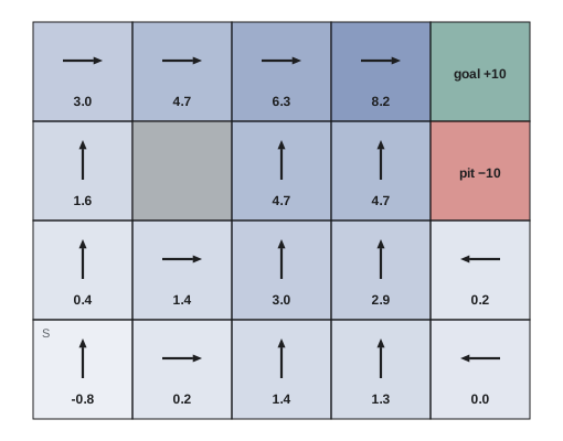
    print(" ".join(row))

value iteration converged in 20 sweeps
>  3.0 >  4.7 >  6.3 >  8.2   G
^  1.6   #    ^  4.7 ^  4.7   X
^  0.4 >  1.4 ^  3.0 ^  2.9 <  0.2
^ -0.8 >  0.2 ^  1.4 ^  1.3 <  0.0

The arrows show the optimal action in each cell and the numbers its value. With a step cost of −1 and a 20% chance of slipping sideways, the agent heads for the goal along the top row, and the cells next to the pit point away from it: in the second row, the agent next to the pit moves up rather than right, accepting a longer route to avoid a 10% chance of slipping into the pit. In the bottom-right corner, the agent moves left rather than up, since moving up passes beside the pit. The policy accounts for risk without any explicit rule, because the values encode expected returns.

Asynchronous DP and generalized policy iteration

DP need not sweep all states systematically. Asynchronous DP updates states in any order, as long as every state continues to be updated, and still converges. This allows focusing computation on the states that matter: those visited by the agent, those near recent changes (prioritized sweeping), or those relevant to the current decision (real-time DP). Learning methods carry this further by updating only states the agent actually experiences.

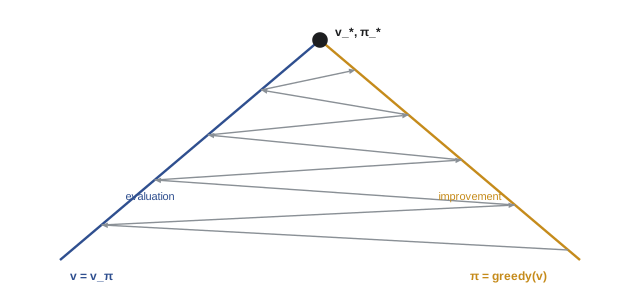
Policy iteration, value iteration and almost all RL methods share a common structure, generalized policy iteration (GPI): a value function is driven toward the value of the current policy (evaluation), and the policy is driven toward being greedy with respect to the value function (improvement). The two processes compete, since improving the policy makes the value function inaccurate and correcting the values may make the policy no longer greedy, but they converge jointly to the optimal value function and an optimal policy. Methods differ in how much evaluation they do before improving, and in whether they use a model, samples or function approximation.

The curse of dimensionality

DP's cost per sweep is roughly \(O(|\mathcal S|^2|\mathcal A|)\) for dense transitions, or \(O(|\mathcal S||\mathcal A|b)\) where \(b\) is the number of possible successor states. This is polynomial in the number of states, much better than searching all \(|\mathcal A|^{|\mathcal S|}\) policies. The problem is that the number of states itself grows exponentially with the number of state variables: a robot arm with 7 joints, each discretized into 100 positions and 100 velocities, has \(10^{28}\) states. Bellman called this the curse of dimensionality. Backgammon has about \(10^{20}\) states and Go about \(10^{170}\), far beyond any table.

Two further obstacles block direct use of DP: the model is often unknown, and even when it exists (a simulator), it may only produce samples rather than explicit probabilities. Lessons 5 to 12 address both. Sample-based methods learn from experience without a model and concentrate on states that actually occur, and function approximation generalizes from visited states to similar unvisited ones.

Lesson 4 examines how to formulate the MDPs that dynamic programming solves, and Lesson 6 shows how planning with learned models brings these ideas to problems where the model must be learned.