Bandits and Markov decision processes

Supervised learning learns from examples labeled with the right answer. Many important problems have no such labels: a robot learning to walk, a program learning to play Go, a system choosing which advertisement to show, a controller tuning a data center's cooling plant, or a language model being refined from human preferences. In each, an agent acts, observes the consequences, and receives a numerical reward signal that says how well it is doing, often long after the actions that mattered. Reinforcement learning (RL) is the study of how to learn good behavior from such interaction. Two features make it distinctive: the agent must explore to discover which actions are good, at the cost of not exploiting what it already knows, and rewards may be delayed, so the agent must work out which earlier actions deserve credit.

This course builds RL from its foundations. This lesson introduces multi-armed bandits, where the exploration problem appears in its simplest form, and Markov decision processes, the mathematical framework for sequential decisions. Later lessons cover dynamic programming, learning from experience, planning, deep RL, policy gradients, model-based and offline RL, multi-agent learning and RL for language models; the section at the end of this lesson shows how they fit together. The course builds on the probability and machine learning of AI-210 and AI-320 and the optimization of AI-310.

Multi-armed bandits

A \(k\)-armed bandit is a repeated choice among \(k\) actions (arms). Each action \(a\) gives a random reward from an unknown distribution with mean \(q_*(a)\), the action's value. The goal is to maximize the total reward over many steps, for example \(T = 1000\). If the values were known, the agent would always pick the best arm; since they are not, it must estimate them from experience while choosing actions.

The natural estimate is the sample average of the rewards received from each action, which can be updated incrementally without storing past rewards:

This "new estimate = old estimate + step size × (target − old estimate)" form recurs throughout RL. With a constant step size \(\alpha\) instead of \(1/n\), the estimate becomes an exponentially weighted average that tracks changing (non-stationary) values.

Exploration versus exploitation

Always choosing the action with the highest current estimate, the greedy action, exploits current knowledge but can lock onto a mediocre arm forever if early samples happened to be unlucky for the best arm. Exploration, trying actions that currently look worse, improves the estimates at a short-term cost. Several strategies balance the two:

• ε-greedy: choose the greedy action with probability \(1 - \varepsilon\) and a random action with probability \(\varepsilon\) (for example 0.1). Simple and robust, but it explores blindly, wasting trials on actions already known to be poor.
• Upper confidence bound (UCB): choose the action maximizing \(Q_t(a) + c\sqrt{\ln t/N_t(a)}\), where \(N_t(a)\) is the number of times \(a\) has been chosen. The bonus is large for rarely tried actions, implementing "optimism in the face of uncertainty"; it shrinks as an action is sampled.
• Thompson sampling: maintain a posterior distribution over each action's value (Lesson 1 of AI-320), sample one value from each posterior, and choose the action with the highest sample. Actions are chosen in proportion to the probability that they are optimal, which explores efficiently and adapts naturally to the evidence.

Performance is measured by regret: the total reward lost relative to always choosing the best arm, \(\mathrm{Regret}_T = Tq_*(a^*) - \sum_t \mathbb{E}[R_t]\). Greedy methods can have regret that grows linearly in \(T\); UCB and Thompson sampling achieve regret that grows only logarithmically, which is optimal.

import numpy as np

rng = np.random.default_rng(0)
K, T, runs = 10, 2000, 200

def run(method, p):
    Q = np.zeros(K); N = np.zeros(K); a_s = np.ones(K); b_s = np.ones(K)
    total = 0.0; optimal = 0
    best = p.argmax()
    for t in range(1, T + 1):
        if method == "greedy":
            a = int(np.argmax(Q + 1e-9 * rng.random(K)))
        elif method == "eps-greedy":
            a = int(rng.integers(K)) if rng.random() < 0.1 else int(np.argmax(Q + 1e-9 * rng.random(K)))
        elif method == "UCB":
            a = t - 1 if t <= K else int(np.argmax(Q + np.sqrt(2 * np.log(t) / N)))
        else:                                    # Thompson sampling with Beta posteriors
            a = int(np.argmax(rng.beta(a_s, b_s)))
        r = float(rng.random() < p[a])
        N[a] += 1; Q[a] += (r - Q[a]) / N[a]     # incremental sample average
        a_s[a] += r; b_s[a] += 1 - r
        total += r; optimal += a == best
    return total / T, optimal / T, p.max() * T - total

for method in ["greedy", "eps-greedy", "UCB", "Thompson"]:
    res = np.array([run(method, rng.uniform(0.1, 0.9, K)) for _ in range(runs)])
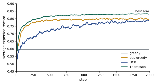
    print(f"{method:10s}  average reward {res[:, 0].mean():.3f}   optimal arm {res[:, 1].mean():5.1%}   regret {res[:, 2].mean():6.1f}")

greedy      average reward 0.613   optimal arm 22.0%   regret  427.3
eps-greedy  average reward 0.779   optimal arm 65.6%   regret  101.6
UCB         average reward 0.735   optimal arm 45.2%   regret  191.3
Thompson    average reward 0.805   optimal arm 72.6%   regret   50.3

The greedy method finds the best arm in only about a fifth of the problems and loses the most reward. ε-greedy does far better, and Thompson sampling, which uses its uncertainty most efficiently, does best, with the lowest regret. UCB with this standard bonus explores more than necessary over 2000 steps; its constant \(c\) is often tuned in practice. Bandit algorithms are widely used for A/B testing, recommendation, advertising and clinical trial design, where each choice has a real cost.

Contextual bandits

In many applications, the best action depends on a context observed before choosing: a user's profile and history determine which article they will click. Contextual bandits learn a policy mapping contexts to actions, typically by modeling the expected reward of each action as a function of the context, for example with linear models (LinUCB) or neural networks, combined with UCB or Thompson exploration. They sit between bandits and full RL: actions affect the immediate reward but not future contexts.

Markov decision processes

In full RL, actions also affect the future: they change the state of the world, and so the rewards available later. The standard model is the Markov decision process (MDP), defined by:

• A set of states \(\mathcal S\) and actions \(\mathcal A\).
• Transition probabilities \(p(s' \mid s, a)\), the probability of moving to state \(s'\) after taking action \(a\) in state \(s\).
• A reward function, giving the expected reward \(r(s, a)\) (or a distribution of rewards) for each transition.
• A discount factor \(\gamma \in [0, 1]\).

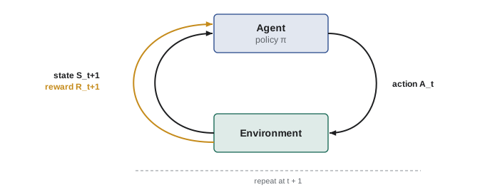
The agent and environment interact in a loop: at time \(t\) the agent observes state \(S_t\), chooses action \(A_t\), and the environment returns reward \(R_{t+1}\) and next state \(S_{t+1}\). The Markov property says that the next state and reward depend only on the current state and action, not on the earlier history; the state must summarize everything relevant about the past. When the agent cannot observe the full state (a robot with noisy sensors, a poker player who cannot see other hands), the problem is a partially observable MDP, which agents handle by maintaining a belief state or a memory of past observations.

Returns and discounting

The agent's goal is to maximize the expected return, the cumulative future reward. For a task with episodes that end (a game, a robot reaching a goal), the return is the sum of rewards until the end. For continuing tasks, rewards are discounted:

Discounting keeps the return finite (for bounded rewards, \(|G_t| \le R_{\max}/(1 - \gamma)\)) and expresses a preference for earlier rewards. The effective horizon is about \(1/(1 - \gamma)\) steps: \(\gamma = 0.99\) looks roughly 100 steps ahead. The recursive form \(G_t = R_{t+1} + \gamma G_{t+1}\) is the seed of everything that follows.

Designing the reward is itself a crucial and difficult step. The agent maximizes exactly what it is rewarded for, so rewards should express the goal, such as winning or reaching a target, rather than hints about how to achieve it, which the agent may exploit in unintended ways. A cleaning robot rewarded for not seeing dirt might learn to close its eyes. This problem of reward misspecification is a central concern of AI safety (AI-430).

Policies and value functions

A policy \(\pi(a \mid s)\) gives the probability of taking each action in each state; a deterministic policy picks one action per state. The value of a state under a policy is the expected return when starting there and following the policy:

The action-value function \(q_\pi\) gives the expected return after taking action \(a\) in state \(s\) and following \(\pi\) thereafter. Using the recursive form of the return, value functions satisfy the Bellman equation:

The value of a state is the expected immediate reward plus the discounted value of the next state. For a finite MDP and a fixed policy, this is a system of linear equations, \(\mathbf v_\pi = \mathbf r_\pi + \gamma P_\pi\mathbf v_\pi\), with solution \(\mathbf v_\pi = (I - \gamma P_\pi)^{-1}\mathbf r_\pi\).

import numpy as np

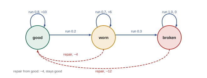
# Machine maintenance MDP. States: 0 good, 1 worn, 2 broken. Actions: 0 run, 1 repair.
# P[a][s, s2] transition probabilities; R[a][s] expected reward for taking a in s.
P = {0: np.array([[0.8, 0.2, 0.0],
                  [0.0, 0.7, 0.3],
                  [0.0, 0.0, 1.0]]),
     1: np.array([[1.0, 0.0, 0.0],
                  [1.0, 0.0, 0.0],
                  [1.0, 0.0, 0.0]])}
R = {0: np.array([10.0, 6.0, 0.0]),       # production profit; a broken machine earns nothing
     1: np.array([-4.0, -4.0, -12.0])}    # repair cost (a breakdown repair costs more)
gamma = 0.95

def evaluate(policy):                     # solve V = R_pi + gamma P_pi V exactly
    P_pi = np.array([P[policy[s]][s] for s in range(3)])
    R_pi = np.array([R[policy[s]][s] for s in range(3)])
    return np.linalg.solve(np.eye(3) - gamma * P_pi, R_pi)

for name, pol in [("repair only when broken", [0, 0, 1]),
                  ("repair when worn", [0, 1, 1]),
                  ("always repair", [1, 1, 1])]:
    V = evaluate(pol)
    print(f"{name:24s}  V(good) = {V[0]:7.2f}  V(worn) = {V[1]:7.2f}  V(broken) = {V[2]:7.2f}")

repair only when broken   V(good) =  132.62  V(worn) =  114.88  V(broken) =  113.98
repair when worn          V(good) =  155.29  V(worn) =  143.53  V(broken) =  135.53
always repair             V(good) =  -80.00  V(worn) =  -80.00  V(broken) =  -88.00

Repairing a worn machine before it breaks is worth more than waiting for a breakdown, because breakdowns cost more to fix and produce nothing until repaired, and repairing a good machine every step is disastrous. Solving the Bellman equations ranks the policies exactly. The next question is how to find the best policy without trying every one; there are \(|\mathcal A|^{|\mathcal S|}\) deterministic policies, far too many for realistic problems.

Optimality

A policy is better than another if its value is at least as high in every state. There is always at least one optimal policy \(\pi_*\), better than or equal to all others, and all optimal policies share the optimal value functions \(v_*(s) = \max_\pi v_\pi(s)\) and \(q_*(s, a) = \max_\pi q_\pi(s, a)\). These satisfy the Bellman optimality equations:

Once \(q_*\) is known, acting optimally is easy: choose \(\arg\max_a q_*(s, a)\) in each state, a greedy policy with respect to the optimal values. Because \(q_*\) already accounts for all future consequences, greedy one-step choices are optimal in the long run. The max makes the optimality equations non-linear, so they are solved iteratively, by dynamic programming when the model is known (Lesson 3) and by learning from experience when it is not (Lessons 5 to 12).

Where RL is used

RL methods have achieved superhuman play in Go, chess, poker and complex video games; control robots and industrial processes; optimize chip placement, compilers and data center cooling; schedule resources; and, through reinforcement learning from human feedback and related methods, shape the behavior of large language models (AI-410). In practice, RL is most successful when a good simulator is available, so that the agent can gather vast experience cheaply and safely, when rewards can be specified well, and when exploration in the real world can be constrained to be safe.

How this course is organized

The twelve lessons build from the simplest decision problems to modern applications:

• Lesson 1 (this lesson): bandits, Markov decision processes, value functions and optimality.
• Lesson 2: bandits in depth: regret bounds, non-stationarity, contextual bandits and off-policy evaluation.
• Lesson 3: dynamic programming: policy evaluation, policy iteration and value iteration.
• Lesson 4: formulating problems: states, rewards and shaping, discounting, constraints and POMDPs.
• Lesson 5: Monte Carlo and temporal-difference learning, SARSA and Q-learning.
• Lesson 6: planning and learning with Dyna and Monte Carlo tree search, up to AlphaZero and MuZero.
• Lesson 7: function approximation, the deadly triad and deep Q-networks.
• Lesson 8: exploration and distributional reinforcement learning.
• Lesson 9: policy gradients, actor-critic methods, PPO and continuous control.
• Lesson 10: model-based and offline reinforcement learning.
• Lesson 11: imitation, inverse reinforcement learning and multi-agent learning.
• Lesson 12: reinforcement learning for language models, safety, and a cooling control project.