Imitation, inverse RL and multi-agent reinforcement learning

Reinforcement learning as described so far assumes a single agent, a reward function supplied by the designer, and learning by trial and error. Each assumption is often violated. Sometimes it is far easier to show the desired behavior than to write down a reward for it: a person can demonstrate driving or folding laundry much more easily than they can specify what makes it good. And many environments contain other learning agents, in games, markets, traffic and teams of robots, whose behavior changes as they learn. This lesson covers learning from demonstrations (behavior cloning and its failure modes, DAgger), inferring rewards from behavior (inverse reinforcement learning and adversarial imitation), and the main ideas of multi-agent reinforcement learning, from game theory to self-play and centralized training.

Behavior cloning

The simplest way to learn from demonstrations is behavior cloning: treat the expert's state-action pairs as a supervised learning data set and train a policy to predict the expert's action in each state. It needs no reward, no environment interaction during training, and only standard supervised learning tools. Early autonomous driving (ALVINN in 1989, which steered a van from camera images) and many modern robot manipulation systems use it, often with large data sets of teleoperated demonstrations.

Behavior cloning has a fundamental weakness, compounding errors. A classifier trained on expert data is accurate on the states the expert visits. But no learner is perfect: a small mistake moves it to a state slightly different from any in the data, where its predictions are less reliable, so it makes further mistakes and drifts further away, into states the expert never visited and from which it never learned to recover. The training and test distributions differ because the learner's own actions shape the states it sees. Ross and Bagnell showed that with a per-step error rate \(\varepsilon\) on the expert's distribution, the total cost over a horizon \(T\) can grow as \(\varepsilon T^2\), rather than the \(\varepsilon T\) one would expect from independent mistakes.

DAgger: dataset aggregation

DAgger fixes the distribution mismatch by collecting expert labels on the states the learner actually visits:

• Train an initial policy on the expert demonstrations.
• Run the current policy in the environment and record the states it visits.
• Ask the expert what action it would take in each of those states.
• Add these labeled states to the data set, retrain on the aggregate, and repeat.

After a few iterations, the data cover the states the learner is likely to reach, including those it reaches after its own mistakes, and the policy learns how to recover. DAgger reduces the error growth to roughly linear in the horizon. Its requirement is an expert who can be queried on arbitrary states, which is easy when the expert is a planning algorithm or a privileged policy in simulation, and harder (but possible with interfaces for corrections) when the expert is a person.

import numpy as np

rng = np.random.default_rng(11)
# Driving down a corridor: lateral position y in -5..5, action -1, 0 or +1. The expert steers toward the centre.
T, ys = 100, range(-5, 6)
expert = lambda y: -int(np.sign(y))
def act(table, y):
    if rng.random() < 0.1:                             # the learner makes a mistake 10% of the time
        return int(rng.integers(-1, 2))
    return table.get(y, int(rng.integers(-1, 2)))      # unseen state: it has no idea, so it guesses
def rollout(table):
    y, cost, visited = 0, 0, []
    for _ in range(T):
        visited.append(y)
        y = int(np.clip(y + act(table, y), -5, 5)); cost += abs(y)
    return cost / T, visited

# Behaviour cloning: the expert always drives in the centre, so the data only contain y = 0
bc_table = {0: expert(0)}
bc = np.mean([rollout(bc_table)[0] for _ in range(500)])
# DAgger: run the current learner, have the expert label every state it visits, aggregate and refit
table = dict(bc_table)
for it in range(3):
    for _ in range(10):
        for y in rollout(table)[1]: table[y] = expert(y)
dag = np.mean([rollout(table)[0] for _ in range(500)])
print(f"states with expert labels: behaviour cloning {sorted(bc_table)}, DAgger {sorted(table)}")
print(f"average distance from the centre per step: behaviour cloning {bc:.2f}, DAgger {dag:.2f}, expert 0.00")

states with expert labels: behavior cloning [0], DAgger [-5, -4, -3, -2, -1, 0, 1, 2, 3, 4, 5]
average distance from the center per step: behavior cloning 1.20, DAgger 0.07, expert 0.00

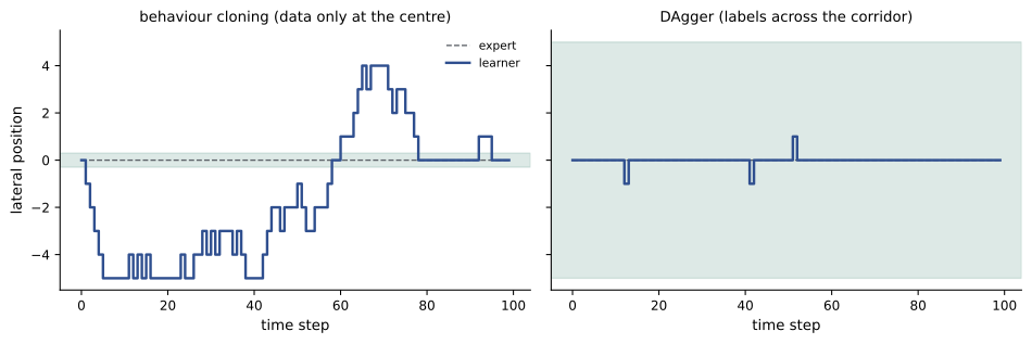
The behavior cloning data contain only the center of the corridor, because that is where the expert always drives. After its first mistake, the cloned policy has no idea what to do and wanders, averaging more than one unit from the center. DAgger, by labeling the states the learner actually reaches, covers the whole corridor and keeps the learner close to the center, despite the same 10% error rate.

Other remedies for compounding errors include injecting noise into the expert's demonstrations so that the data include recoveries (DART), training on augmented data with perturbed states, predicting chunks of future actions rather than single actions, and using expressive policy classes, such as diffusion policies, that model multimodal expert behavior without averaging distinct strategies into an invalid compromise.

Inverse reinforcement learning

Imitation copies behavior; inverse reinforcement learning (IRL) tries to recover the reward function that explains it. Given demonstrations from an expert assumed to be acting (near-)optimally, IRL searches for a reward under which the expert's behavior is optimal. A recovered reward can transfer to new situations where copying actions would not work, for example a different vehicle or a changed environment, and can be inspected to understand what the expert values.

IRL is ill-posed: many rewards make the same behavior optimal, including the trivial reward of zero everywhere. Approaches resolve the ambiguity in different ways:

• Feature matching (Abbeel and Ng): assume the reward is linear in features of the state, \(r(s) = \mathbf{w}^\top\boldsymbol\phi(s)\), and find a policy whose expected discounted feature counts match the expert's; any such policy performs as well as the expert under any reward in the class.
• Maximum entropy IRL (Ziebart): among all trajectory distributions that match the expert's feature counts, choose the one with maximum entropy, which gives trajectories probability proportional to the exponential of their reward, \(p(\tau) \propto e^{R(\tau)}\). This handles suboptimal, noisy demonstrations gracefully and leads to a convex likelihood for linear rewards.
• Bayesian IRL: place a prior over rewards and compute a posterior given the demonstrations.

Generative adversarial imitation learning (GAIL) skips recovering an explicit reward. A discriminator is trained to distinguish expert state-action pairs from the learner's, and the learner is trained with RL, using the discriminator's output as its reward, to fool it. At equilibrium, the learner's state-action distribution matches the expert's. GAIL is more robust to compounding errors than behavior cloning, because it learns from its own trajectories, but it requires environment interaction and inherits the instability of adversarial training.

Multi-agent reinforcement learning

When several agents learn in a shared environment, each agent's environment includes the others, whose policies keep changing. From any one agent's point of view the environment is non-stationary, which breaks the assumptions behind single-agent convergence results. Multi-agent problems are framed as stochastic (Markov) games: a state, a joint action of all agents, transitions depending on the joint action, and a reward for each agent. They divide by the relationship between agents:

• Fully cooperative: all agents share one reward, as in a team of warehouse robots or a fleet of traffic signals. The challenge is coordination and credit assignment: which agent's action caused the team reward?
• Fully competitive (zero-sum): one agent's gain is the other's loss, as in chess, Go and poker.
• Mixed (general-sum): agents have partly aligned and partly conflicting interests, as in markets, negotiation and traffic.

Game-theoretic solution concepts

In multi-agent settings there is usually no single optimal policy, because the best policy depends on what others do. The central concept is the Nash equilibrium: a profile of policies in which no agent can gain by changing its own policy while the others keep theirs. In two-player zero-sum games, Nash equilibria coincide with minimax strategies and guarantee each player at least the game's value whatever the opponent does. Equilibria often require randomization: in rock-paper-scissors, the only equilibrium is to play each action with probability 1/3, since any predictable pattern can be exploited.

Learning dynamics do not necessarily converge to equilibria. Naive independent learners in rock-paper-scissors chase each other in cycles. No-regret algorithms, however, have a powerful guarantee: if each player uses an algorithm whose average regret goes to zero, the time-averaged strategies converge to equilibrium in two-player zero-sum games (and to coarse correlated equilibria in general games).

import numpy as np

# Regret matching in rock-paper-scissors self-play. Payoff for the row player: win +1, loss -1.
P = np.array([[0, -1, 1], [1, 0, -1], [-1, 1, 0]])
rng = np.random.default_rng(12)
regret = [np.array([5.0, 0.0, 0.0]), np.zeros(3)]       # player 1 starts biased toward rock
avg = [np.zeros(3), np.zeros(3)]
for t in range(1, 20001):
    strat = []
    for p in range(2):
        pos = np.maximum(regret[p], 0)
        strat.append(pos / pos.sum() if pos.sum() > 0 else np.ones(3) / 3)
    a = [rng.choice(3, p=strat[0]), rng.choice(3, p=strat[1])]
    u0 = P[:, a[1]]; u1 = -P[a[0], :]                # payoff of each action against the choice of the opponent
    regret[0] += u0 - u0[a[0]]; regret[1] += u1 - u1[a[1]]
    avg[0] += strat[0]; avg[1] += strat[1]
    if t in (10, 100, 1000, 20000):
        print(f"after {t:5d} rounds: player 1 average strategy {np.round(avg[0] / t, 3)}, current {np.round(strat[0], 2)}")

after    10 rounds: player 1 average strategy [0.744 0.18  0.076], current [0.27 0.36 0.36]
after   100 rounds: player 1 average strategy [0.37  0.237 0.393], current [0. 0. 1.]
after  1000 rounds: player 1 average strategy [0.312 0.328 0.359], current [0. 1. 0.]
after 20000 rounds: player 1 average strategy [0.322 0.337 0.341], current [0.32 0.68 0.  ]

The current strategy swings between pure actions throughout, but the time average approaches (1/3, 1/3, 1/3), the Nash equilibrium. Counterfactual regret minimization (CFR) extends regret matching to games with hidden information and sequential moves by minimizing regret separately at each information set; CFR variants with abstraction and real-time search produced the first programs to beat top professionals at heads-up no-limit Texas hold'em (Libratus, 2017) and six-player poker (Pluribus, 2019).

Self-play and populations

In competitive games, an agent can train against copies of itself, generating an endless curriculum of opponents that improve as it does, as in TD-Gammon, AlphaZero (Lesson 6) and OpenAI Five for Dota 2. Pure self-play can cycle or overfit to its own quirks, forgetting how to beat strategies it no longer sees. Population-based methods train against a league of past and diverse agents: AlphaStar, which reached grandmaster level in StarCraft II, used a league including exploiter agents whose sole purpose was to find weaknesses in the main agents.

Cooperative MARL

For cooperative teams, fully centralized control (one agent choosing the joint action) does not scale, because the joint action space grows exponentially with the number of agents, and fully independent learning ignores coordination. The dominant compromise is centralized training with decentralized execution (CTDE): during training, a centralized critic sees all agents' observations and actions, which stabilizes learning and helps assign credit, while at execution each agent acts on its own observations. Examples include MADDPG and MAPPO (a multi-agent version of PPO with a centralized value function, Lesson 9). Value decomposition methods such as VDN and QMIX learn a team Q-value as a sum or monotonic combination of individual agents' Q-values, so that each agent's greedy action is consistent with the team's greedy joint action. Difference rewards, which compare the team reward with what it would have been without one agent's action, address credit assignment directly.