Visualization and communication

Visualization serves two different purposes in a data project. Exploratory visualization is for the analyst: dozens of quick, rough plots made to understand the data, find errors and form hypotheses before any model is built. Explanatory visualization is for an audience: a few carefully designed charts that communicate a finding or a decision clearly and honestly. The first is about speed and breadth; the second about clarity, accuracy and the reader.

This lesson starts with why summary statistics are not enough, then covers how people read charts, choosing the right chart, exploratory analysis in practice, honest presentation and uncertainty, color and accessibility, and communicating model results to people who will act on them.

Why look at the data

In 1973 the statistician Francis Anscombe published four small data sets with nearly identical summary statistics: the same means and variances of x and y, the same correlation and the same fitted regression line. Plotted, they look completely different: one is a noisy linear relationship, one a smooth curve, one a perfect line with a single outlier, and one a vertical stack of points with a single extreme point that creates the whole correlation.

import numpy as np

x123 = [10, 8, 13, 9, 11, 14, 6, 4, 12, 7, 5]
data = {
    "I":   (x123, [8.04, 6.95, 7.58, 8.81, 8.33, 9.96, 7.24, 4.26, 10.84, 4.82, 5.68]),
    "II":  (x123, [9.14, 8.14, 8.74, 8.77, 9.26, 8.10, 6.13, 3.10, 9.13, 7.26, 4.74]),
    "III": (x123, [7.46, 6.77, 12.74, 7.11, 7.81, 8.84, 6.08, 5.39, 8.15, 6.42, 5.73]),
    "IV":  ([8, 8, 8, 8, 8, 8, 8, 19, 8, 8, 8],
            [6.58, 5.76, 7.71, 8.84, 8.47, 7.04, 5.25, 12.50, 5.56, 7.91, 6.89]),
}
print("set  mean_x  var_x  mean_y  var_y   corr   fitted line")
for name, (x, y) in data.items():
    x, y = np.array(x, float), np.array(y)
    slope, intercept = np.polyfit(x, y, 1)
    print(f"{name:>3}  {x.mean():6.2f} {x.var(ddof=1):6.2f} {y.mean():7.2f} {y.var(ddof=1):6.2f}"
          f" {np.corrcoef(x, y)[0, 1]:6.3f}   y = {intercept:.2f} + {slope:.3f}x")

set  mean_x  var_x  mean_y  var_y   corr   fitted line
  I    9.00  11.00    7.50   4.13  0.816   y = 3.00 + 0.500x
 II    9.00  11.00    7.50   4.13  0.816   y = 3.00 + 0.500x
III    9.00  11.00    7.50   4.12  0.816   y = 3.00 + 0.500x
 IV    9.00  11.00    7.50   4.12  0.817   y = 3.00 + 0.500x

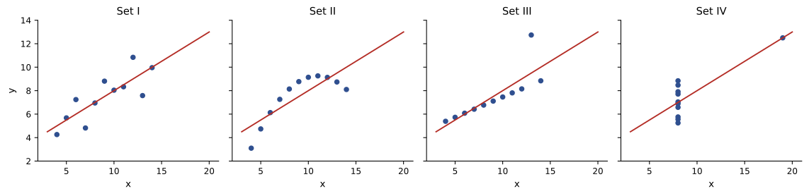
A model fit to any of these sets would produce the same line, and only set I would justify it. The lesson generalizes: summary statistics, and model metrics, compress data and can hide exactly the structure that matters. Plot distributions, relationships and errors before trusting a number.

How people read charts

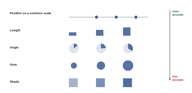
A chart encodes numbers as visual properties, and people decode some properties far more accurately than others. Experiments by William Cleveland and Robert McGill in the 1980s, since repeated many times, rank the common encodings from most to least accurate roughly as follows:

• Position along a common scale (dots or bar ends against a shared axis).
• Position along identical but unaligned scales (small multiples).
• Length, then direction and angle (pie slices).
• Area, then volume, curvature and color saturation or hue.

The practical rule is to encode the most important comparison with position on a common axis. A bar chart beats a pie chart for comparing parts, because lengths along a shared baseline are judged more accurately than angles; a dot plot or line chart beats a bubble chart for comparing values, because areas are systematically misjudged. Color hue is excellent for distinguishing categories but poor for showing quantities.

Choosing a chart

The question the chart must answer decides its type:

• Comparing categories: a bar chart (horizontal if labels are long), sorted by value unless the categories have a natural order. A dot plot works well for many categories or when the baseline is not zero.
• Change over time: a line chart, with time on the horizontal axis. Bars suit a few discrete periods.
• Distribution of one variable: a histogram or density plot; box plots or violin plots to compare distributions across groups.
• Relationship between two variables: a scatter plot, with transparency or hexagonal binning when there are thousands of points.
• Parts of a whole: a stacked bar, or a pie chart with no more than about three slices whose exact values do not matter.
• Many variables: a correlation heatmap, a scatter-plot matrix, or small multiples (a grid of identical small charts, one per group).
• Geography: a choropleth map for rates by region (never raw counts, which mostly show where people live), or points on a map.

Small multiples deserve special mention. Instead of overlaying ten lines in ten colors, draw ten small charts with the same axes; the eye compares shapes across panels easily, and no legend is needed.

Exploratory analysis

Exploratory data analysis (EDA) follows a rough sequence: look at each variable alone (distributions, missing values, outliers), then at pairs (relationships with the target, correlations between features), then at groups and time (does the relationship differ by segment or change over time?). The code below produces a typical first set of plots for a numeric target.

import numpy as np
import pandas as pd
import matplotlib.pyplot as plt

rng = np.random.default_rng(4)
n = 800
df = pd.DataFrame({"size_m2": rng.gamma(6, 18, n), "age": rng.integers(0, 70, n),
                   "type": rng.choice(["condo", "house", "townhouse"], n, p=[0.4, 0.4, 0.2])})
base = {"condo": 3200, "house": 2600, "townhouse": 2900}
df["price"] = (df["type"].map(base) * df["size_m2"] * (1 - 0.004 * df["age"])
               * rng.lognormal(0, 0.15, n)).round(-3)

fig, ax = plt.subplots(1, 3, figsize=(12, 3.6))
ax[0].hist(df["price"] / 1000, bins=40, color="#2f4f8f")
ax[0].set(title="Price distribution", xlabel="price ($ thousands)", ylabel="homes")
groups = ["condo", "townhouse", "house"]
ax[1].boxplot([df.loc[df.type == g, "price"] / 1000 for g in groups], tick_labels=groups)
ax[1].set(title="Price by type", ylabel="price ($ thousands)")
ax[2].scatter(df["size_m2"], df["price"] / 1000, s=8, alpha=0.35, color="#1c6b58")
ax[2].set(title="Price vs size", xlabel="size (m²)", ylabel="price ($ thousands)")
fig.tight_layout()
fig.savefig("eda.svg")

print(df[["size_m2", "age", "price"]].describe().round(0).loc[["mean", "50%", "max"]])
print(f"skew of price: {df.price.skew():.2f}; of log price: {np.log(df.price).skew():.2f}")

      size_m2   age     price
mean    108.0  35.0  272751.0
50%     100.0  34.0  249500.0
max     322.0  69.0  936000.0
skew of price: 1.07; of log price: -0.34

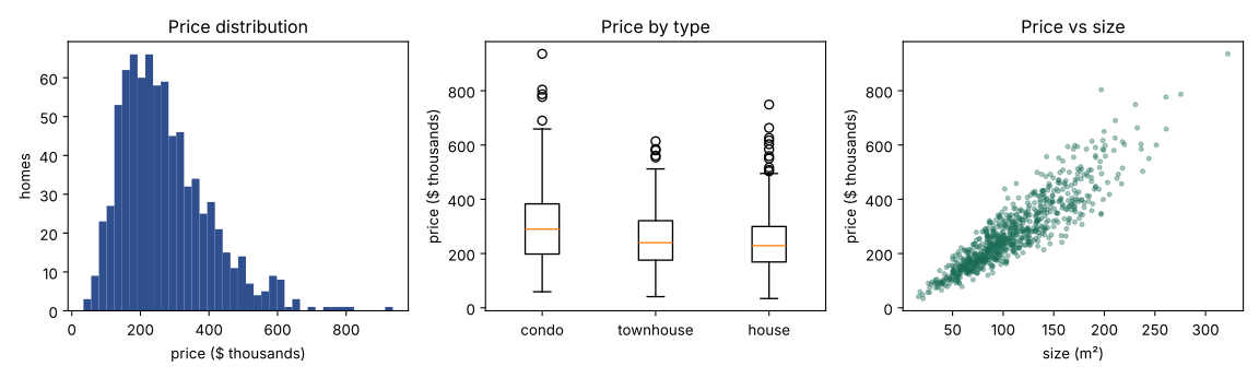
The plots suggest modeling decisions: the long right tail and the fanning scatter both suggest predicting log price, and the overlapping box plots show that type alone explains little until size is accounted for.

Honest charts

Charts can mislead even when every number is correct. The most common distortions are:

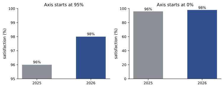
• Truncated axes on bar charts: a bar's length encodes its value, so the axis must start at zero. Line charts and dot plots, which encode position, may use a non-zero baseline if it is clearly labeled.
• Inconsistent or dual axes: two series with independently scaled vertical axes can be made to appear correlated, or to cross, at will.
• Cherry-picked ranges: starting a time series at a convenient low or high point.
• Area and 3-D effects: doubling a pictogram's height also doubles its width, so the area quadruples; 3-D perspective distorts the values of nearer and farther bars.
• Raw counts where rates are needed: more cases in larger regions or larger groups say nothing about risk.

Edward Tufte's lie factor quantifies distortion: the size of the effect shown in the graphic divided by the size of the effect in the data. An honest chart has a lie factor close to 1.

Showing uncertainty

Every estimate from data has uncertainty, and a chart that shows a point estimate alone invites over-confident readings. Ways to show it include error bars or shaded bands for confidence intervals, showing the individual data points behind a summary, and showing distributions rather than averages. The bootstrap is a general way to compute intervals without formulas: resample the data with replacement many times, recompute the statistic each time, and take the middle 95% of the results.

import numpy as np

rng = np.random.default_rng(21)
a = rng.exponential(30, 60)       # session minutes, variant A (60 users)
b = rng.exponential(36, 60)       # variant B

def boot_ci(x, n=5000):
    means = rng.choice(x, size=(n, len(x)), replace=True).mean(axis=1)
    return np.percentile(means, [2.5, 97.5])

diffs = (rng.choice(b, (5000, 60)).mean(axis=1) - rng.choice(a, (5000, 60)).mean(axis=1))
for name, x in [("A", a), ("B", b)]:
    lo, hi = boot_ci(x)
    print(f"{name}: mean {x.mean():5.1f} min, 95% CI {lo:5.1f} to {hi:5.1f}")
lo, hi = np.percentile(diffs, [2.5, 97.5])
print(f"B - A: {b.mean() - a.mean():5.1f} min, 95% CI {lo:5.1f} to {hi:5.1f}")

A: mean  29.1 min, 95% CI  22.2 to  36.9
B: mean  38.1 min, 95% CI  29.6 to  47.6
B - A:   8.9 min, 95% CI  -2.9 to  20.8

Variant B's average looks higher, but the interval for the difference includes zero, so 60 users per variant cannot establish that B is better. A bar chart of the two means without intervals would have suggested a clear winner.

Color and accessibility

Color should have a job. Use a qualitative palette (distinct hues) for categories, a sequential palette (light to dark in one hue) for ordered quantities, and a diverging palette (two hues meeting at a neutral midpoint) for values above and below a meaningful center, such as change from last year. Rainbow palettes, which run through many hues, create false boundaries where hues change and are not ordered perceptually.

About 8% of men and 0.5% of women have some form of color vision deficiency, most often difficulty distinguishing red from green. Palettes designed for color-blind readers (such as Okabe-Ito, or the viridis family for sequential data) avoid relying on red-green contrast. Better still, do not rely on color alone: label lines directly at their ends instead of using a legend, use different marker shapes or line styles, and make sure the chart still works in grayscale.

Charts published on the web should also be accessible to readers who use screen readers: provide a text alternative that states what the chart shows and its key finding, and make the underlying data available as a table. In the US, Section 508 of the Rehabilitation Act requires federal agencies' electronic content to meet the Web Content Accessibility Guidelines (WCAG), and a 2024 Department of Justice rule under the Americans with Disabilities Act requires state and local governments' web content to meet WCAG 2.1 level AA, which includes text alternatives and sufficient contrast.

Communicating results

A chart for an audience should answer one question, and its title should state the answer: "Churn fell after the price change" rather than "Monthly churn rate". Remove everything that does not help the reader decode the data (heavy gridlines, borders, shading, 3-D effects, redundant legends), label directly, and highlight the one series or bar that matters with color while graying out the rest.

When presenting a model, translate metrics into the audience's terms. "AUC 0.87" means little to an operations manager; "if we review the 500 highest-risk claims each week, we expect to catch about 70% of fraudulent claims, and about one in four reviewed claims will be fraudulent" supports a decision. Show performance for the groups the audience cares about, and state the limitations: what data the model has not seen, how it might fail, and how it will be monitored.

Dashboards bring many charts together for ongoing monitoring. A good dashboard is built for specific decisions and users, puts the most important figures at the top left, shows comparisons (to targets, to last period) rather than isolated numbers, keeps the same scales across related panels, and shows when the data was last updated. A dashboard nobody acts on should be retired.

Lesson 11 applies these principles to recurring metrics and dashboards, and to the design and analysis of experiments.