
AI-220 · Lesson 8 of 12 · 30 min
Data pipelines and storage
A notebook that cleans a CSV once is an analysis. A system that collects, validates, transforms and stores data every day, reliably, for months, is a data pipeline, and building it is the core of data engineering. Machine learning systems depend on pipelines twice: to produce training data, and to produce the same features at prediction time. When the two disagree, models fail silently in production, a problem called training-serving skew.
This lesson covers where data is stored (databases, warehouses, lakes and file formats), how pipelines move and transform it (ETL and ELT, batch and streaming), the engineering properties that make pipelines reliable (idempotency, incremental loads, validation, orchestration), and how data is versioned and traced.
Operational and analytical stores
Data lives in two kinds of system with opposite designs:
- Operational (OLTP, online transaction processing) databases, such as PostgreSQL and MySQL, run applications. They handle many small reads and writes of individual records, enforce constraints and transactions, and store data row by row so that a whole record can be read or updated quickly. They are normalized: each fact is stored once, in tables linked by keys.
- Analytical (OLAP, online analytical processing) stores, such as data warehouses (Snowflake, BigQuery, Amazon Redshift) and query engines over files, answer questions over many records: total sales by region by month, or the features of every customer last year. They store data column by column, compress it heavily and scan it in parallel.
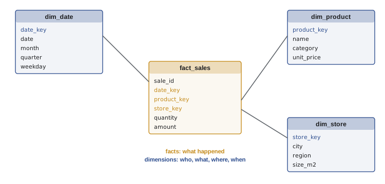
Analytical tables are often organized as a star schema: a central fact table recording events or measurements (each sale, with quantity and price) surrounded by dimension tables describing the entities involved (products, stores, dates, customers). Queries join the fact table to the dimensions they need and aggregate.
import sqlite3

con = sqlite3.connect(":memory:")
con.executescript("""
CREATE TABLE dim_product (product_key INTEGER PRIMARY KEY, name TEXT, category TEXT);
CREATE TABLE dim_store   (store_key INTEGER PRIMARY KEY, city TEXT);
CREATE TABLE fact_sales  (sale_id INTEGER PRIMARY KEY, sale_date TEXT,
                          product_key INTEGER REFERENCES dim_product,
                          store_key INTEGER REFERENCES dim_store,
                          quantity INTEGER, amount REAL);
INSERT INTO dim_product VALUES (1, 'kettle', 'kitchen'), (2, 'toaster', 'kitchen'), (3, 'lamp', 'lighting');
INSERT INTO dim_store VALUES (1, 'Ottawa'), (2, 'Winnipeg');
INSERT INTO fact_sales VALUES
  (1, '2026-04-01', 1, 1, 2, 79.98), (2, '2026-04-01', 3, 2, 1, 45.00),
  (3, '2026-04-02', 2, 1, 1, 34.99), (4, '2026-05-03', 1, 2, 3, 119.97),
  (5, '2026-05-04', 3, 1, 4, 180.00), (6, '2026-05-04', 2, 2, 2, 69.98);
""")
query = """
SELECT substr(f.sale_date, 1, 7) AS month, p.category, s.city,
       SUM(f.quantity) AS units, ROUND(SUM(f.amount), 2) AS revenue
FROM fact_sales f
JOIN dim_product p USING (product_key)
JOIN dim_store s USING (store_key)
GROUP BY month, p.category, s.city
ORDER BY month, revenue DESC
"""
for row in con.execute(query):
print(row)('2026-04', 'kitchen', 'Ottawa', 3, 114.97)
('2026-04', 'lighting', 'Winnipeg', 1, 45.0)
('2026-05', 'kitchen', 'Winnipeg', 5, 189.95)
('2026-05', 'lighting', 'Ottawa', 4, 180.0)Files, lakes and formats
Large volumes of raw data, logs, images and model training sets are usually kept as files in object storage (Amazon S3, Azure Blob Storage, Google Cloud Storage), which is cheap, durable and nearly unlimited. A collection of such files organized for analysis is called a data lake. Table formats such as Apache Iceberg and Delta Lake add database features on top of files, including transactions, schema changes and the ability to query a table as it was at an earlier time, a combination often called a lakehouse.
The file format matters a great deal:
| Format | Layout | Schema | Strengths | Weaknesses |
|---|---|---|---|---|
| CSV | Rows, text | None (all text) | Universal, human-readable | Large, slow, no types, quoting problems |
| JSON lines | Rows, text | Self-describing | Nested data, API output | Large, slow to parse |
| Avro | Rows, binary | Embedded | Streaming, schema evolution | Not efficient for analytics |
| Parquet | Columns, binary | Embedded | Compression, reads only needed columns, statistics for skipping | Not human-readable, poor for single-row updates |
Columnar formats like Parquet store all values of one column together. A query that needs 3 of 60 columns reads roughly 5% of the data, and similar values stored together compress far better than mixed rows. Parquet also stores the minimum and maximum of each column for each block of rows, so a query for one day's data can skip blocks whose date range does not include it.
Files are usually partitioned into folders by a column that queries filter on, most often date: sales/date=2026-05-04/part-0.parquet. A query for May reads only May's folders. Partitions should be large enough (typically hundreds of megabytes per file) that the overhead of many small files does not dominate.
Worked problem
Storage and scan cost
An application produces 2 TB of raw JSON logs per day. Converted to Parquet they compress 8:1. They are kept 400 days in object storage at $0.023 per GB-month. A daily report reads 4 of the 50 columns for the last 30 days, and the query engine charges $5 per TB scanned. Find the steady-state storage cost per month and the report's cost per run, with and without Parquet.
Show solution
- Raw JSON stored: \(2 \times 400 = 800\) TB = 800,000 GB; cost \(800{,}000 \times 0.023 = \$18{,}400\) per month.
- Parquet: 100 TB stored; cost $2300 per month.
- Report on JSON: reads all 30 days in full: \(2 \times 30 = 60\) TB; cost $300 per run.
- Report on Parquet: 30 days is 7.5 TB; reading 4 of 50 columns reads about \(7.5 \times 4/50 = 0.6\) TB; cost $3 per run.
Answer: Parquet cuts storage from about $18,400 to $2,300 a month and the daily report from about $300 to $3 (roughly $9,000 a month to $90). Format and layout decisions are among the largest cost levers in data engineering.
import gzip, io
import numpy as np
import pandas as pd

rng = np.random.default_rng(0)
n = 200_000
df = pd.DataFrame({
    "country": rng.choice(["CA", "US", "MX"], n),
    "device":  rng.choice(["ios", "android", "web"], n, p=[0.3, 0.5, 0.2]),
    "ms":      rng.integers(20, 900, n),
})
csv = df.to_csv(index=False).encode()
print(f"CSV {len(csv) / 1e6:.1f} MB, gzip-compressed {len(gzip.compress(csv)) / 1e6:.1f} MB")

as_text = df.memory_usage(deep=True).sum() / 1e6
cat = df.astype({"country": "category", "device": "category", "ms": "int16"})
print(f"in memory: {as_text:.1f} MB as text columns, {cat.memory_usage(deep=True).sum() / 1e6:.1f} MB with categories and int16")CSV 2.6 MB, gzip-compressed 0.5 MB in memory: 22.6 MB as text columns, 0.8 MB with categories and int16
The same ideas apply in memory: storing a low-cardinality text column as a category (an integer code per row plus one copy of each distinct value) and using the smallest adequate integer type cut memory use by more than an order of magnitude here.
ETL and ELT
A pipeline extracts data from sources, transforms it (cleaning, joining, aggregating, computing features) and loads it into a store. Two orderings are common:
- ETL (extract, transform, load): data is transformed in a separate processing step before loading into the warehouse. Traditional, and still used where the destination should hold only cleaned data or where transformation needs code that the warehouse cannot run.
- ELT (extract, load, transform): raw data is loaded first and transformed inside the warehouse with SQL, usually managed by a tool such as dbt that versions the SQL models, tests them and builds them in dependency order. ELT keeps the raw data available for reprocessing and is now the most common pattern for analytics.
Pipelines are also either batch or streaming. Batch pipelines process data in scheduled chunks (hourly, daily) and are simpler and cheaper. Streaming pipelines process events continuously as they arrive, through a message system such as Apache Kafka, and are needed when predictions or alerts must reflect events within seconds, as in fraud detection. Many systems combine them: a streaming path for fresh features and a batch path that recomputes everything accurately overnight.
Making pipelines reliable
Idempotency and backfills
A pipeline step is idempotent if running it twice on the same input produces the same result as running it once. This matters because steps fail and are retried, and because pipelines are rerun to fix bugs or process history (a backfill). A step that appends rows each time it runs creates duplicates on every retry; a step that replaces the partition for its date, or upserts on a key, does not.
import sqlite3

con = sqlite3.connect(":memory:")
con.execute("CREATE TABLE daily (day TEXT, store INTEGER, revenue REAL, PRIMARY KEY (day, store))")

def load_day(day, rows, append=False):
    with con:                                   # one transaction: all or nothing
        if not append:
            con.execute("DELETE FROM daily WHERE day = ?", (day,))
        con.executemany("INSERT OR REPLACE INTO daily VALUES (?, ?, ?)" if not append
                        else "INSERT INTO daily VALUES (?, ?, ?)", [(day, s, r) for s, r in rows])

rows = [(1, 520.0), (2, 310.5)]
for attempt in range(3):                        # the scheduler retries the same day 3 times
    load_day("2026-05-04", rows)
print("idempotent load:", con.execute("SELECT COUNT(*), SUM(revenue) FROM daily").fetchone())

con.execute("DROP TABLE daily")
con.execute("CREATE TABLE daily (day TEXT, store INTEGER, revenue REAL)")
for attempt in range(3):
    load_day("2026-05-04", rows, append=True)
print("append-only load:", con.execute("SELECT COUNT(*), SUM(revenue) FROM daily").fetchone())idempotent load: (2, 830.5) append-only load: (6, 2491.5)
Incremental loads
Reprocessing all history every day becomes too slow as data grows. An incremental pipeline processes only what has changed since the last run, tracked by a watermark: the latest timestamp (or id) already processed. Each run reads records newer than the watermark, processes them and then advances it. Late-arriving records, such as events from a phone that was offline, are handled by reprocessing a window behind the watermark (for example the last three days) on each run, which works only because the load step is idempotent.
Validation
A pipeline should check its data at every boundary rather than trusting its sources. Typical checks are schema (expected columns and types), volume (row counts within an expected range of yesterday's), completeness (null rates), validity (ranges, allowed values), uniqueness of keys, referential integrity (every product key exists in the product table) and freshness (the newest record is recent). Failed records can be quarantined for inspection while the rest proceeds, or the whole run can be stopped, depending on how harmful bad data would be. Tools such as dbt tests and Great Expectations express these checks declaratively.
import pandas as pd

def validate(df, expected_rows):
    problems = []
    required = {"order_id", "customer_id", "amount", "ts"}
    if missing := required - set(df.columns):
        return [f"missing columns {sorted(missing)}"]
    if not 0.5 * expected_rows <= len(df) <= 1.5 * expected_rows:
        problems.append(f"row count {len(df)} outside expected range around {expected_rows}")
    if df["order_id"].duplicated().any():
        problems.append(f"{df.order_id.duplicated().sum()} duplicate order_id")
    if (null_rate := df["customer_id"].isna().mean()) > 0.01:
        problems.append(f"customer_id null rate {null_rate:.0%}")
    bad = ~df["amount"].between(0, 10_000)
    if bad.any():
        problems.append(f"{bad.sum()} amounts out of range: {df.loc[bad, "amount"].tolist()}")
    return problems

batch = pd.DataFrame({
    "order_id": [1, 2, 3, 3, 5, 6],
    "customer_id": [10, 11, None, 12, 13, 14],
    "amount": [25.0, -4.0, 18.5, 18.5, 99_999.0, 40.0],
    "ts": pd.date_range("2026-05-04", periods=6, freq="h"),
})
for p in validate(batch, expected_rows=6) or ["all checks passed"]:
print("-", p)- 1 duplicate order_id - customer_id null rate 17% - 2 amounts out of range: [-4.0, 99999.0]
Orchestration
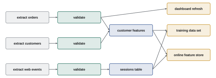
A real pipeline has many steps with dependencies: the feature table cannot be built until today's orders and customer updates have loaded. Orchestrators such as Apache Airflow, Dagster and Prefect represent the pipeline as a directed acyclic graph (DAG) of tasks, run each task when its upstream tasks succeed, retry failures, record every run, and support backfills over date ranges. A DAG makes the pipeline's structure explicit and lets a failed step be rerun without repeating everything before it.
Features for training and serving
Features must be computed the same way for training (from history, in batch) and for serving (for one entity, at request time, in milliseconds). Writing the logic twice, once in SQL for training and once in application code for serving, almost guarantees that they will drift apart. A feature store addresses this by defining each feature once and materializing it in two places: an offline store with full history for building point-in-time correct training sets, and an online store (a low-latency key-value database) holding the latest values for serving. Models that use embeddings, such as retrieval systems, also need a vector database or vector index that can find the nearest embeddings to a query quickly.
Versioning and lineage
A model is a function of its code and its data, so reproducing it needs both. Code is versioned with Git; data needs its own versioning, because data sets are too large for Git and change over time. Tools such as DVC store data in object storage and keep a small pointer file, containing a content hash, in Git; table formats such as Iceberg and Delta Lake keep a history of table snapshots. Either way, a training run should record exactly which version of each data set it used.
import hashlib
import pandas as pd

def snapshot_id(df):
    """A stable fingerprint of a data frame contents and column order."""
    h = hashlib.sha256()
    h.update(",".join(df.columns).encode())
    h.update(pd.util.hash_pandas_object(df, index=False).values.tobytes())
    return h.hexdigest()[:12]

v1 = pd.DataFrame({"id": [1, 2, 3], "label": ["cat", "dog", "cat"]})
v2 = v1.copy(); v2.loc[2, "label"] = "dog"          # one label corrected
v1_again = pd.DataFrame({"id": [1, 2, 3], "label": ["cat", "dog", "cat"]})

print("v1      ", snapshot_id(v1))
print("v1 again", snapshot_id(v1_again))
print("v2 ", snapshot_id(v2))v1 cfc05c85b1da v1 again cfc05c85b1da v2 f8978b62bac4
Lineage records where each data set came from: which sources and transformations produced it and which downstream tables and models depend on it. It answers questions such as "which models were trained on the table with the bad currency conversion?" and is needed for debugging, audits and honoring deletion requests.
Where data is stored can be a legal question. In the US there is no general data residency requirement for private companies, but federal agencies require cloud services to be authorized under FedRAMP, criminal justice information must meet the FBI's CJIS Security Policy, health data stored by a vendor requires a HIPAA business associate agreement, and contracts with customers or foreign privacy laws (such as the EU GDPR) often restrict where data may be processed.
Lesson 9 continues with processing data that does not fit on one machine, and Lesson 12 with contracts, drift and skew monitoring for pipelines that feed production models.
Common mistakes
MistakeRunning analytics directly on the production database.
InsteadCopy data to an analytical store so heavy queries do not slow the application.
MistakeStoring large analytical data sets as CSV.
InsteadUse a columnar, compressed format such as Parquet, partitioned by common filter columns.
MistakeWriting pipeline steps that append on every run.
InsteadMake steps idempotent: replace partitions or upsert on keys, inside a transaction.
MistakeTrusting source data because it came from an internal system.
InsteadValidate schema, volume, nulls, ranges, keys and freshness at every pipeline boundary.
MistakeReimplementing feature logic separately for serving.
InsteadDefine features once (for example in a feature store) to avoid training-serving skew.
MistakeTraining a model without recording the data version.
InsteadVersion data with content hashes or table snapshots and record them with each training run.
Summary and key terms
- OLTP databases store rows for transactions; OLAP warehouses store columns for analysis, often in a star schema of facts and dimensions.
- Data lakes keep files in object storage; table formats (Iceberg, Delta Lake) add transactions and time travel.
- Parquet is columnar, compressed and skippable; partition files by date or other filter columns.
- ETL transforms before loading; ELT loads raw data and transforms in the warehouse, often with dbt.
- Batch pipelines are simpler; streaming pipelines (via Kafka) serve low-latency needs.
- Idempotent steps (replace or upsert, in transactions) make retries and backfills safe; watermarks enable incremental loads.
- Validate schema, volume, completeness, validity, uniqueness, integrity and freshness at every boundary.
- Orchestrators run pipelines as DAGs with retries, logging and backfills.
- Feature stores keep training and serving features consistent; version data and record lineage for reproducibility.
- OLTP
- Online transaction processing: systems handling many small reads and writes of individual records.
- OLAP
- Online analytical processing: systems for queries that aggregate many records.
- Data warehouse
- A managed analytical database storing data in columnar form.
- Data lake
- A store of files in object storage organized for analysis.
- Star schema
- A fact table of events joined by keys to dimension tables describing entities.
- Parquet
- A compressed, columnar file format with embedded schema and statistics.
- Partitioning
- Dividing data into separate files or folders by a column value such as date.
- ELT
- Extract, load, transform: loading raw data and transforming it inside the warehouse.
- Idempotent
- Producing the same result whether run once or many times.
- Backfill
- Running a pipeline over historical periods.
- Watermark
- The marker of the latest data already processed by an incremental pipeline.
- DAG
- Directed acyclic graph: tasks with dependencies and no cycles.
- Feature store
- A system that defines features once and serves them consistently for training and prediction.
- Training-serving skew
- A difference between features computed for training and for prediction.
- Data lineage
- The record of the sources and transformations behind each data set.
Practice problems
Work each problem on paper first, then reveal the answer to check.
Why are operational databases stored by rows and warehouses by columns?
Show answer
Transactions read and write whole records, which rows make fast; analytical queries read a few columns across many records, which columns make fast and compressible.
A table has 80 columns of similar size. A query needs 6. Roughly what fraction of a Parquet file is read, before compression and block skipping?
Show answer
6/80 = 7.5%.
Logs of 500 GB per day are kept for 365 days at $0.023 per GB-month after 6:1 compression. What is the monthly storage cost?
Show answer
500 × 365 / 6 = 30,417 GB; × 0.023 = about $700 per month.
A pipeline step runs "INSERT INTO sales SELECT * FROM staging". Why is it not idempotent, and how could it be fixed?
Show answer
Each rerun inserts the rows again. Delete the target partition (or rows with the batch's keys) first, or use an upsert (MERGE / INSERT OR REPLACE) on a primary key, inside a transaction.
An incremental pipeline uses a watermark on event time. Events arrive up to 48 hours late. What should each run process?
Show answer
All events with event time after (watermark − 48 h), reloading those periods idempotently, then advance the watermark.
Yesterday's batch had 1.2 million rows; today's has 40,000. What should the pipeline do?
Show answer
Fail the volume check and alert, rather than publishing a table missing most of the day's data; investigate the source.
Draw (or list) the dependencies for: extract orders, extract products, validate each, join into sales, build features, train model.
Show answer
extract orders → validate orders; extract products → validate products; both validations → join sales → build features → train model.
What is training-serving skew, and give an example.
Show answer
A difference between how features are computed in training and at prediction time, e.g. "average order value" computed over 90 days in SQL for training but over 30 days in the app at serving time.
Why is a content hash better than a file name for identifying a data set version?
Show answer
File names can be reused for changed data; the hash changes whenever the contents change and is identical for identical contents.
When is streaming worth its complexity?
Show answer
When decisions must reflect events within seconds or minutes, such as fraud detection, real-time recommendations or monitoring; otherwise batch is simpler and cheaper.
Lesson quiz · 5 questions
Score 60% or more to complete this lesson.
Create a free account to save your progress, take quizzes and earn a certificate.