Cleaning and feature engineering

Raw data is never ready for a model. Values are missing, categories are spelled five ways, units are mixed, dates arrive as text, the same record appears twice and a few values are physically impossible. Cleaning turns that raw data into a consistent table; feature engineering then turns the cleaned columns into inputs a model can learn from. Both are full of judgment calls, and both can quietly introduce leakage if they are done on the whole data set before it is split.

This lesson works through a realistic cleaning pass, then treats outliers and missing values, the main feature transformations, and finally scikit-learn pipelines, which make the whole process reproducible and leakage-free.

Profile before you clean

The first step is to look. A profile of each column shows its type, the number of missing and distinct values, the most common values and the range. Problems that a profile reveals in seconds, such as a numeric column read as text because of one stray "n/a", can take hours to discover from model errors.

import io
import pandas as pd

raw = """id,city,weight,unit,signup,plan,monthly_fee
1, Toronto ,72,kg,2025-01-04,Basic,10
2,toronto,165,lb,2025-01-09,basic,10
3,Montreal,80,kg,2025-02-30,Pro,25
4,Vancouver,,kg,2025-02-11,PRO,25
5,Montreal,68,kg,2025-03-02,Pro,unknown
5,Montreal,68,kg,2025-03-02,Pro,unknown
6,Calgary,790,kg,2025-03-15,Basic,10
7,Toronto,59,kg,,Basic,10
"""
df = pd.read_csv(io.StringIO(raw))
print(df.dtypes.to_string())
print()
print("missing:", df.isna().sum()[lambda s: s > 0].to_dict())
print("duplicate rows:", df.duplicated().sum())
print("city values:", sorted(df["city"].unique()))
print("plan values:", sorted(df["plan"].unique()))

id               int64
city               str
weight         float64
unit               str
signup             str
plan               str
monthly_fee        str

missing: {'weight': 1, 'signup': 1}
duplicate rows: 1
city values: [' Toronto ', 'Calgary', 'Montreal', 'Toronto', 'Vancouver', 'toronto']
plan values: ['Basic', 'PRO', 'Pro', 'basic']

The profile shows several problems at once: monthly_fee was read as text because of the word "unknown" (pandas treats common markers such as "NA", "n/a" and empty fields as missing automatically, but not arbitrary words); city has inconsistent case and spacing; plan has three spellings of two values; there is a duplicate row; weights mix kilograms and pounds; one date (February 30) is impossible; and a weight of 790 kg is almost certainly an entry error.

A cleaning pass

Each fix should be a deliberate, documented decision, written as code so that it can be rerun on new data:

import io
import numpy as np
import pandas as pd

raw = """id,city,weight,unit,signup,plan,monthly_fee
1, Toronto ,72,kg,2025-01-04,Basic,10
2,toronto,165,lb,2025-01-09,basic,10
3,Montreal,80,kg,2025-02-30,Pro,25
4,Vancouver,,kg,2025-02-11,PRO,25
5,Montreal,68,kg,2025-03-02,Pro,unknown
5,Montreal,68,kg,2025-03-02,Pro,unknown
6,Calgary,790,kg,2025-03-15,Basic,10
7,Toronto,59,kg,,Basic,10
"""
df = pd.read_csv(io.StringIO(raw), na_values=["unknown"])

df = df.drop_duplicates()                                  # exact duplicate rows
df["city"] = df["city"].str.strip().str.title()            # " toronto " -> "Toronto"
df["plan"] = df["plan"].str.lower()                        # one spelling per plan
df.loc[df["unit"] == "lb", "weight"] *= 0.4536             # convert to kg
df = df.drop(columns="unit")
df["signup"] = pd.to_datetime(df["signup"], errors="coerce")   # bad dates -> NaT
df.loc[~df["weight"].between(30, 300), "weight"] = np.nan      # impossible weights -> missing

print(df.to_string(index=False))

 id      city  weight     signup  plan  monthly_fee
  1   Toronto  72.000 2025-01-04 basic         10.0
  2   Toronto  74.844 2025-01-09 basic         10.0
  3  Montreal  80.000        NaT   pro         25.0
  4 Vancouver     NaN 2025-02-11   pro         25.0
  5  Montreal  68.000 2025-03-02   pro          NaN
  6   Calgary     NaN 2025-03-15 basic         10.0
  7   Toronto  59.000        NaT basic         10.0

Notice what was not done: no missing values were filled in, and no rows were dropped except the exact duplicate. Converting impossible values to missing, rather than deleting rows or guessing a correction, keeps the decision about how to handle them for the next step and preserves the rest of the record. In a real project, the 790 kg entry should also be reported back to whoever owns the source system, since a data error found downstream is usually a process error upstream.

Validity rules

Many cleaning checks can be written as rules that every record must satisfy: ranges (weights between 30 and 300 kg), allowed values (plan is basic or pro), formats (postal codes), uniqueness (one row per id) and cross-field consistency (a cancellation date is after the signup date). Writing these rules once and running them on every new batch turns cleaning into data validation, which Lesson 8 builds into pipelines.

Outliers

An outlier is a value far from the rest. Some are errors; others are the most important records in the data set, such as a genuinely large transaction in a fraud model. Two common detection rules are:

• The z-score rule: flag values more than about 3 standard deviations from the mean. It assumes a roughly normal distribution, and the outliers themselves inflate the standard deviation, which can hide them.
• The interquartile range (IQR) rule: with quartiles \(Q_1\) and \(Q_3\) and \(\text{IQR} = Q_3 - Q_1\), flag values below \(Q_1 - 1.5\,\text{IQR}\) or above \(Q_3 + 1.5\,\text{IQR}\). Because quartiles are barely affected by extreme values, it is more robust.

import numpy as np

rng = np.random.default_rng(0)
x = np.append(rng.normal(50, 5, 200), [95, 120])     # 200 normal values + 2 outliers

z = (x - x.mean()) / x.std()
q1, q3 = np.percentile(x, [25, 75])
iqr = q3 - q1
lo, hi = q1 - 1.5 * iqr, q3 + 1.5 * iqr

print(f"mean {x.mean():.1f}, std {x.std():.1f}")
print("z-score > 3:", np.round(x[np.abs(z) > 3], 1))
print(f"IQR fences: {lo:.1f} to {hi:.1f}")
print("IQR outliers:", np.round(x[(x < lo) | (x > hi)], 1))

mean 50.6, std 7.5
z-score > 3: [ 95. 120.]
IQR fences: 37.0 to 63.4
IQR outliers: [ 95. 120.]

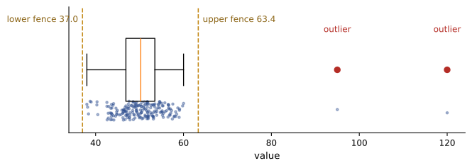
Once detected, an outlier can be corrected (if the true value is known), set to missing (if it is an error), capped at a limit (winsorizing), transformed (a log transform pulls in long right tails), or kept. Models based on trees are largely insensitive to extreme input values, while linear models and neural networks are strongly affected by them.

Missing values

How to handle missing values depends on why they are missing:

• Missing completely at random (MCAR): missingness is unrelated to anything, as when a sensor drops random readings. Dropping or simple imputation introduces little bias.
• Missing at random (MAR): missingness depends on other observed variables, as when older customers more often skip an online form field. Imputing from those variables can correct for it.
• Missing not at random (MNAR): missingness depends on the missing value itself, as when people with high incomes decline to report income. No imputation from the data can fully fix this, and the fact of missingness is itself informative.

Common strategies are to drop rows (acceptable only if few rows are affected and the data is MCAR), to impute a constant such as the median, to impute from a group (the median for the same city or product type), or to impute with a model that predicts the missing value from other columns. Whatever the method, adding a binary indicator column ("weight_missing") lets the model learn whether missingness itself predicts the target.

import numpy as np
import pandas as pd

rng = np.random.default_rng(1)
n = 1000
group = rng.choice(["a", "b"], size=n)
value = np.where(group == "a", rng.normal(20, 3, n), rng.normal(40, 3, n))
df = pd.DataFrame({"group": group, "value": value})
true_std = df["value"].std()

mask = rng.random(n) < np.where(group == "b", 0.4, 0.05)   # MAR: group b far more often missing
df.loc[mask, "value"] = np.nan

overall = df["value"].fillna(df["value"].median())
by_group = df["value"].fillna(df.groupby("group")["value"].transform("median"))

print(f"missing: {df.value.isna().mean():.1%}")
print(f"true mean {value.mean():.2f}  std {true_std:.2f}")
print(f"drop rows mean {df.value.mean():.2f}")
print(f"overall-median mean {overall.mean():.2f}  std {overall.std():.2f}")
print(f"group-median mean {by_group.mean():.2f}  std {by_group.std():.2f}")

missing: 20.8%
true mean 29.85  std 10.58
drop rows mean 27.85
overall-median mean 26.81  std 9.38
group-median mean 29.78  std 10.38

Because values in group b, which are larger, are missing far more often, dropping rows and imputing the overall median both pull the mean well below the truth. Imputing within each group recovers the mean almost exactly. Any single-value imputation shrinks the spread, because every filled value sits at the center, which is why some analyses use multiple imputation, filling each gap several times with random draws.

Feature engineering

Features are the inputs a model sees. Good features expose the structure of the problem in a form the model can use; for linear models and many neural networks this often matters more than the choice of algorithm. Common transformations include:

• Scaling: standardization \(z = (x - \mu)/\sigma\) gives each feature mean 0 and standard deviation 1; min-max scaling maps to [0, 1]. Distance-based methods (k-nearest neighbors, clustering), regularized linear models and neural networks need scaled inputs; tree-based models do not.
• Log and power transforms: incomes, prices and counts often have long right tails; \(\log(1 + x)\) makes them more symmetric and turns multiplicative effects into additive ones.
• Encoding categories: one-hot encoding creates one binary column per category. For high-cardinality categories (thousands of values), alternatives include grouping rare values into "other", hashing, target encoding (below) and learned embeddings.
• Dates and times: day of week, hour, month, holiday flags, time since an event. Cyclical features such as hour of day can be encoded as \(\sin(2\pi h/24)\) and \(\cos(2\pi h/24)\) so that 23:00 and 01:00 are close.
• Ratios, differences and aggregates: price per square meter, debt to income, a customer's number of orders in the last 30 days. Aggregates over time must respect point-in-time correctness (Lesson 1).
• Interactions and domain knowledge: a feature that experts know matters, such as body mass index from weight and height.

import numpy as np
import pandas as pd

df = pd.DataFrame({
    "price": [120_000, 250_000, 1_400_000, 310_000],
    "area_m2": [60, 95, 240, 110],
    "type": ["condo", "house", "house", "townhouse"],
    "listed": pd.to_datetime(["2026-01-05 09:00", "2026-01-14 23:00", "2026-02-20 01:00", "2026-03-08 14:00"]),
})
feat = pd.DataFrame({
    "log_price": np.log1p(df["price"]).round(2),
    "price_per_m2": (df["price"] / df["area_m2"]).round(0),
    "weekday": df["listed"].dt.day_name().str[:3],
    "hour_sin": np.sin(2 * np.pi * df["listed"].dt.hour / 24).round(2),
    "hour_cos": np.cos(2 * np.pi * df["listed"].dt.hour / 24).round(2),
})
feat = pd.concat([feat, pd.get_dummies(df["type"], prefix="type", dtype=int)], axis=1)
print(feat.to_string(index=False))

 log_price  price_per_m2 weekday  hour_sin  hour_cos  type_condo  type_house  type_townhouse
     11.70        2000.0     Mon      0.71     -0.71           1           0               0
     12.43        2632.0     Wed     -0.26      0.97           0           1               0
     14.15        5833.0     Fri      0.26      0.97           0           1               0
     12.64        2818.0     Sun     -0.50     -0.87           0           0               1

The hour encoding places 23:00 (sin −0.26, cos 0.97) and 01:00 (sin 0.26, cos 0.97) close together, as they should be, whereas the raw hours 23 and 1 are far apart.

Fit on training data only

Every transformation that learns something from the data, such as a mean for imputation or scaling, the categories for one-hot encoding, or the mean target per category for target encoding, must be learned from the training set alone and then applied unchanged to the validation and test sets. Learning it from the whole data set leaks information about the test set into training, so the measured performance overstates what the model will achieve on new data.

Target encoding shows the danger most clearly. It replaces each category with the average target value for that category. Computed on all the data, it gives each test record a feature built partly from its own label. The example below uses a category that has no relationship to the target at all, yet the leaked encoding makes it look predictive.

import numpy as np
import pandas as pd
from sklearn.linear_model import LogisticRegression
from sklearn.metrics import roc_auc_score
from sklearn.model_selection import train_test_split

rng = np.random.default_rng(0)
n = 4000
df = pd.DataFrame({"cat": rng.integers(0, 1500, n),        # 1500 categories, no signal
                   "y": rng.integers(0, 2, n)})
train, test = train_test_split(df, test_size=0.5, random_state=0)

def evaluate(enc_source):
    means = enc_source.groupby("cat")["y"].mean()
    prior = train["y"].mean()
    enc = lambda d: d["cat"].map(means).fillna(prior).to_frame()
    model = LogisticRegression().fit(enc(train), train["y"])
    return roc_auc_score(test["y"], model.predict_proba(enc(test))[:, 1])

print(f"encoding fit on ALL data:   test AUC = {evaluate(df):.3f}")
print(f"encoding fit on train only: test AUC = {evaluate(train):.3f}")

encoding fit on ALL data:   test AUC = 0.846
encoding fit on train only: test AUC = 0.519

An AUC of 0.5 means no predictive power. The leaked version looks like a useful model even though the category is pure noise. Even when fit on training data only, target encoding of rare categories overfits the training set, so practitioners compute it out-of-fold (each training row encoded using the other folds) and shrink rare categories toward the overall mean.

Pipelines

Scikit-learn pipelines package the cleaning and feature steps with the model, so that fitting the pipeline fits every step on the training data, and predicting applies the same fitted steps to new data. A ColumnTransformer applies different steps to different columns. Pipelines prevent leakage during cross-validation (each fold refits the transformations), make the preprocessing part of the saved model, and guarantee that training and serving use the same code.

import numpy as np
import pandas as pd
from sklearn.compose import ColumnTransformer
from sklearn.impute import SimpleImputer
from sklearn.linear_model import LogisticRegression
from sklearn.model_selection import cross_val_score
from sklearn.pipeline import make_pipeline
from sklearn.preprocessing import OneHotEncoder, StandardScaler

rng = np.random.default_rng(5)
n = 600
X = pd.DataFrame({
    "income": rng.lognormal(11, 0.5, n),
    "age": rng.integers(18, 80, n).astype(float),
    "region": rng.choice(["n", "s", "e", "w"], n),
})
logit = 0.00004 * (X["income"] - 60000) - 0.03 * (X["age"] - 45) + (X["region"] == "e") * 1.0
y = (rng.random(n) < 1 / (1 + np.exp(-logit))).astype(int)
X.loc[rng.random(n) < 0.1, "income"] = np.nan                 # 10% missing income

numeric = make_pipeline(SimpleImputer(strategy="median", add_indicator=True), StandardScaler())
categorical = OneHotEncoder(handle_unknown="ignore")
prep = ColumnTransformer([("num", numeric, ["income", "age"]), ("cat", categorical, ["region"])])
model = make_pipeline(prep, LogisticRegression(max_iter=1000))

scores = cross_val_score(model, X, y, cv=5, scoring="roc_auc")
print("fold AUCs:", np.round(scores, 3))
print(f"mean AUC: {scores.mean():.3f}")
model.fit(X, y)
print("features after preprocessing:", list(model[0].get_feature_names_out()))

fold AUCs: [0.764 0.794 0.798 0.857 0.763]
mean AUC: 0.795
features after preprocessing: ['num__income', 'num__age', 'num__missingindicator_income', 'cat__region_e', 'cat__region_n', 'cat__region_s', 'cat__region_w']

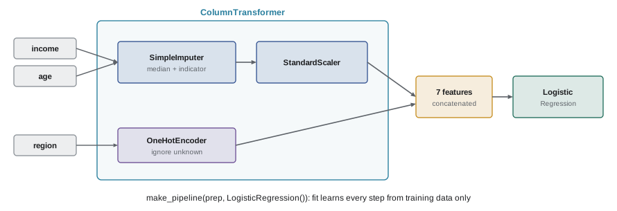
The pipeline imputes median income with a missing-value indicator, standardizes the numeric columns, one-hot encodes region (ignoring regions unseen in training) and fits the model, all inside each cross-validation fold. The fitted pipeline can be saved and loaded as a single object for serving (AI-410).

Lesson 5 extends these methods to text, time series, location and image data, each of which needs its own cleaning and features.