Machine learning with scikit-learn

The previous lessons prepared data; this one learns from it. scikit-learn is Python's standard library for classical machine learning: regression, classification, clustering, preprocessing and model evaluation, all behind one consistent interface. Deep learning frameworks such as PyTorch take over for neural networks on images, audio and text (CMPUT-466, AI-340 and AI-350), but scikit-learn remains the workhorse for tabular data, the rows and columns of business and engineering records, where well-tuned classical models are often as accurate as deep networks and far easier to build, explain and maintain. This lesson shows the workflow end to end: fitting models, splitting data, measuring performance honestly, building pipelines and tuning settings without fooling yourself.

The estimator interface

Every scikit-learn model is an estimator object with the same methods:

• fit(X, y) learns from training data, where X is a two-dimensional array or DataFrame of features (one row per example) and y holds the targets.
• predict(X) returns predictions for new rows; classifiers also offer predict_proba(X), the predicted probability of each class.
• Transformers, such as scalers and encoders, have fit(X) and transform(X) instead, or fit_transform(X) for both.

Learned values are stored as attributes ending in an underscore, such as coef_ and intercept_. Because every model shares this interface, swapping a linear model for a random forest is a one-line change.

import numpy as np
from sklearn.linear_model import LinearRegression
from sklearn.metrics import mean_absolute_error
from sklearn.model_selection import train_test_split

rng = np.random.default_rng(0)
util = rng.uniform(0, 100, 300)                         # CPU utilization, %
watts = 180 + 2.9 * util + rng.normal(0, 15, 300)      # measured server power, W
X = util.reshape(-1, 1)                                 # scikit-learn wants a 2-D feature array

X_train, X_test, y_train, y_test = train_test_split(X, watts, test_size=0.25, random_state=0)
model = LinearRegression().fit(X_train, y_train)

print(f"Idle power {model.intercept_:.0f} W, {model.coef_[0]:.2f} W per % utilization")
print(f"Test MAE: {mean_absolute_error(y_test, model.predict(X_test)):.1f} W")
print("Predicted power at 50% and 90%:", model.predict([[50], [90]]).round(0))

Idle power 180 W, 2.89 W per % utilization
Test MAE: 12.8 W
Predicted power at 50% and 90%: [325. 440.]

The model recovers the idle power (about 180 W) and the slope (about 2.9 W per percentage point of utilization) that generated the data, and its predictions on the 25% of servers it never saw are off by about 13 W on average. That last number, the error on held-out data, is the one that matters.

Why we split the data

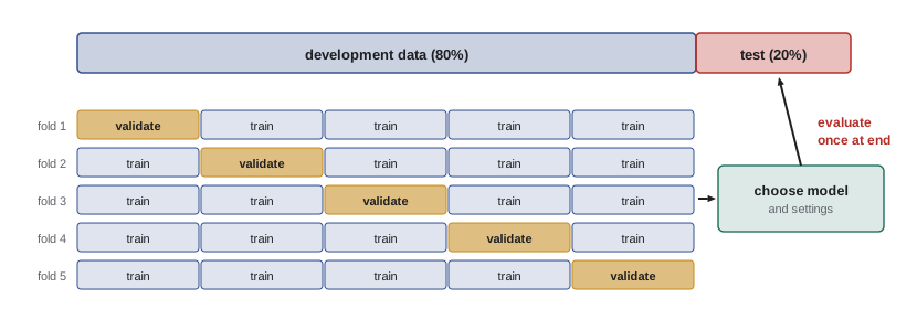
A model is useful only if it works on data it has not seen. Its error on its own training data is optimistic, sometimes wildly so, because a flexible model can memorize the training examples, noise and all. The standard practice is to divide the data:

• a training set to fit the model;
• a validation set (or cross-validation, below) to compare models and choose settings;
• a test set, locked away and used once at the very end to estimate real-world performance.

If the test set is used repeatedly to pick models, it stops being a fair test. For data collected over time, split by time (train on the past, test on the future) rather than randomly, to match how the model will be used and avoid leakage (Lesson 6).

Classification and its metrics

Classification predicts a category: will this disk fail in the next 30 days, is this transaction fraudulent, which of five fault types caused this alarm? Accuracy, the fraction of correct predictions, is the obvious metric and often the wrong one. When one class is rare, a model that always predicts the common class scores very high accuracy while being useless.

The confusion matrix counts true positives (TP), false positives (FP), true negatives (TN) and false negatives (FN). From it:

Precision answers "when the model raises an alarm, how often is it right?"; recall answers "of the real failures, how many did it catch?"

import numpy as np
from sklearn.dummy import DummyClassifier
from sklearn.linear_model import LogisticRegression
from sklearn.metrics import confusion_matrix, precision_score, recall_score
from sklearn.model_selection import train_test_split

rng = np.random.default_rng(1)
n = 5000
realloc = rng.poisson(1.5, n)                # reallocated sectors
temp = rng.normal(38, 5, n)                 # drive temperature, C
age = rng.uniform(0, 6, n)                  # years in service
risk = -8.0 + 1.1 * realloc + 0.12 * (temp - 38) + 0.5 * age
fails = rng.random(n) < 1 / (1 + np.exp(-risk))   # failed within 30 days
X = np.column_stack([realloc, temp, age])
print(f"Failure rate: {fails.mean():.1%}")

X_tr, X_te, y_tr, y_te = train_test_split(X, fails, test_size=0.3, random_state=1, stratify=fails)
for name, clf in [("always predict OK", DummyClassifier(strategy="most_frequent")),
                  ("logistic regression", LogisticRegression(max_iter=1000))]:
    pred = clf.fit(X_tr, y_tr).predict(X_te)
    print(f"{name:>20}: accuracy {np.mean(pred == y_te):.3f}, recall {recall_score(y_te, pred, zero_division=0):.2f}")

proba = LogisticRegression(max_iter=1000).fit(X_tr, y_tr).predict_proba(X_te)[:, 1]
for threshold in [0.5, 0.2, 0.1]:
    pred = proba >= threshold
    tn, fp, fn, tp = confusion_matrix(y_te, pred).ravel()
    print(f"threshold {threshold}: caught {tp} of {tp + fn} failures, {fp} false alarms, "
          f"precision {precision_score(y_te, pred, zero_division=0):.2f}")

Failure rate: 2.9%
   always predict OK: accuracy 0.971, recall 0.00
 logistic regression: accuracy 0.973, recall 0.12
threshold 0.5: caught 5 of 43 failures, 3 false alarms, precision 0.62
threshold 0.2: caught 17 of 43 failures, 24 false alarms, precision 0.41
threshold 0.1: caught 24 of 43 failures, 74 false alarms, precision 0.24

Only 2.9% of disks fail, so the baseline that always says "OK" is 97.1% accurate and catches nothing. Logistic regression is barely more accurate at the default threshold of 0.5, but its predicted probabilities are useful: lowering the threshold to 0.2 catches 17 of 43 failures at the cost of 24 false alarms, and 0.1 catches 24 at the cost of 74. The right threshold is a business decision, not a statistical one: it depends on what a missed failure costs compared with an unnecessary disk replacement.

Pipelines and cross-validation

Real data needs preparation: missing values filled, numbers scaled, categories encoded (Lesson 6). If that preparation is done by hand before splitting, information leaks from the validation and test data into training. scikit-learn's Pipeline chains the preparation steps and the model into one estimator, so that every step is fitted on the training portion only, every time. ColumnTransformer applies different preparation to different columns.

k-fold cross-validation splits the development data into k parts (folds), trains on k − 1 and validates on the remaining one, rotating through all k. The average score is a more reliable estimate than a single split, and the spread across folds shows how much it varies.

import numpy as np
import pandas as pd
from sklearn.compose import ColumnTransformer
from sklearn.impute import SimpleImputer
from sklearn.linear_model import Ridge
from sklearn.model_selection import cross_val_score
from sklearn.pipeline import make_pipeline
from sklearn.preprocessing import OneHotEncoder, StandardScaler

rng = np.random.default_rng(3)
n = 400
df = pd.DataFrame({
    "it_mw": rng.uniform(2, 40, n),
    "outside_c": rng.uniform(-20, 35, n),
    "cooling": rng.choice(["air", "liquid", "hybrid"], n),
})
effect = df["cooling"].map({"air": 0.10, "hybrid": 0.06, "liquid": 0.03})
df["pue"] = 1.12 + effect + 0.004 * df["outside_c"].clip(lower=5) + rng.normal(0, 0.015, n)
df.loc[rng.choice(n, 20, replace=False), "outside_c"] = np.nan      # some weather data missing

numeric = make_pipeline(SimpleImputer(strategy="median"), StandardScaler())
prep = ColumnTransformer([("num", numeric, ["it_mw", "outside_c"]),
                          ("cat", OneHotEncoder(handle_unknown="ignore"), ["cooling"])])
model = make_pipeline(prep, Ridge(alpha=1.0))

X, y = df.drop(columns="pue"), df["pue"]
scores = -cross_val_score(model, X, y, cv=5, scoring="neg_mean_absolute_error")
print("MAE in each fold:", scores.round(4))
print(f"Mean MAE {scores.mean():.4f} +/- {scores.std():.4f}")

MAE in each fold: [0.0187 0.0209 0.0184 0.0191 0.0159]
Mean MAE 0.0186 +/- 0.0016

Because the imputer, scaler and encoder sit inside the pipeline, cross_val_score refits them within each fold: the median used to fill missing temperatures in fold 3, for example, is computed without looking at fold 3. The average error is about 0.019 PUE. The noise in the data is 0.015, so a straight-line model is leaving some structure unexplained; the next section shows why.

Underfitting, overfitting and model complexity

Every model family has settings, called hyperparameters, that control its flexibility: the depth of a decision tree, the strength of regularization in a ridge regression, the number of neighbors in k-nearest neighbors. Too little flexibility underfits: the model cannot capture the real pattern, and both training and validation errors are high. Too much overfits: the model fits the noise in the training data, its training error falls toward zero, and its validation error rises.

import numpy as np
from sklearn.model_selection import train_test_split
from sklearn.tree import DecisionTreeRegressor

rng = np.random.default_rng(9)
x = rng.uniform(-15, 35, 600)
y = 1.20 + 0.006 * np.clip(x, 5, None) + rng.normal(0, 0.02, 600)    # PUE with a free-cooling kink
X = x.reshape(-1, 1)
X_tr, X_val, y_tr, y_val = train_test_split(X, y, test_size=0.3, random_state=9)

print("depth  train MAE  validation MAE")
for depth in [1, 2, 3, 5, 8, 12, None]:
    tree = DecisionTreeRegressor(max_depth=depth, random_state=0).fit(X_tr, y_tr)
    tr = np.mean(np.abs(tree.predict(X_tr) - y_tr))
    va = np.mean(np.abs(tree.predict(X_val) - y_val))
    print(f"{str(depth):>5}  {tr:9.4f}  {va:14.4f}")

depth  train MAE  validation MAE
    1     0.0261          0.0254
    2     0.0170          0.0198
    3     0.0151          0.0182
    5     0.0134          0.0191
    8     0.0088          0.0209
   12     0.0034          0.0221
 None     0.0000          0.0240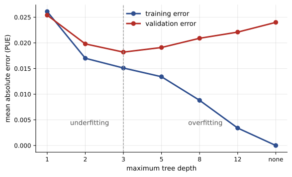

A depth-1 tree (one split) underfits. At depth 3 the validation error is lowest. Beyond that, the training error keeps falling, reaching zero for an unlimited tree that has memorized every training point, while the validation error rises. Choosing the model by training error would pick the worst one.

Tuning hyperparameters

GridSearchCV automates the search: it tries every combination of the listed hyperparameter values, scores each by cross-validation on the development data, and refits the best one on all of it. Only then is the test set used, once, to report final performance.

import numpy as np
from sklearn.ensemble import RandomForestRegressor
from sklearn.model_selection import GridSearchCV, train_test_split

rng = np.random.default_rng(9)
x = rng.uniform(-15, 35, 600)
humidity = rng.uniform(20, 90, 600)
y = 1.20 + 0.006 * np.clip(x, 5, None) + 0.0004 * humidity + rng.normal(0, 0.02, 600)
X = np.column_stack([x, humidity])
X_dev, X_test, y_dev, y_test = train_test_split(X, y, test_size=0.2, random_state=1)

search = GridSearchCV(RandomForestRegressor(n_estimators=100, random_state=0),
                      {"max_depth": [3, 6, None], "min_samples_leaf": [1, 10]},
                      cv=5, scoring="neg_mean_absolute_error")
search.fit(X_dev, y_dev)
print("Best settings:", search.best_params_)
print(f"Cross-validated MAE: {-search.best_score_:.4f}")
test_mae = np.mean(np.abs(search.predict(X_test) - y_test))
print(f"Held-out test MAE:   {test_mae:.4f}")
print("Feature importances (temperature, humidity):", search.best_estimator_.feature_importances_.round(2))

Best settings: {'max_depth': 6, 'min_samples_leaf': 10}
Cross-validated MAE: 0.0163
Held-out test MAE:   0.0169
Feature importances (temperature, humidity): [0.98 0.02]

The random forest, an average of many decision trees each trained on a random sample of the data, captures the kink that the linear model missed. The cross-validated error (0.0163) and the held-out test error (0.0169) agree closely, which is the sign of an honest evaluation. Feature importances show that temperature does nearly all the work and humidity very little, consistent with how the data was generated. Importances are a useful first look but can mislead when features are correlated; Lesson 12 discusses explaining models more carefully.

Choosing a model

A few model families cover most tabular problems:

• Linear and logistic regression: fast, interpretable and a strong baseline; add regularization (ridge, lasso) when there are many features.
• Decision trees: easy to explain but unstable on their own.
• Random forests and gradient-boosted trees (such as scikit-learn's HistGradientBoosting, XGBoost and LightGBM): usually the most accurate choice for tabular data, handling non-linear effects and interactions with little preparation.
• k-nearest neighbors and support vector machines: useful for small data sets with well-scaled features.

Always start with a trivial baseline (predict the mean, or the most common class) and a simple model. Many projects find that a well-prepared simple model is good enough, and every additional bit of complexity must earn its place by beating the baseline on validation data.