Cleaning and preparing data

Surveys of data scientists consistently find that preparing data takes more of their time than modeling it. Real data arrives with inconsistent labels, numbers stored as text, duplicated records, impossible values, ambiguous dates and missing entries. A model trained on such data learns the mess. This lesson builds on the pandas skills of Lesson 5 to give a systematic approach: profile the data to find problems, clean it with explicit and recorded decisions, deal with outliers thoughtfully, prepare features for machine learning without leaking information, and validate every new batch automatically.

Profile before you clean

The first step is to look, not to fix. A quick profile answers: how many rows and columns, what type pandas inferred for each column, how many values are missing, whether any rows are duplicated, and what distinct values the categorical columns hold. Many problems reveal themselves immediately.

import pandas as pd

raw = pd.DataFrame({
    "ticket": ["T1", "T2", "T3", "T3", "T4", "T5", "T6", "T7"],
    "site": ["YYZ-1", "yyz-1 ", "ORD-2", "ORD-2", "SEA-1", "SEA1", "ORD-2", None],
    "opened": ["2026-03-02", "2026-03-04", "2026-03-04", "2026-03-04", "03/09/2026", "2026-03-11", "2026-03-12", "2026-03-15"],
    "hours": ["2.5", "4", "1.5", "1.5", "n/a", "3.0 h", "-1", "6"],
    "cost": [180.0, 320.0, 95.0, 95.0, None, 240.0, 150.0, 51000.0],
})

print(raw.dtypes.to_string())
print("Rows:", len(raw), "| exact duplicate rows:", raw.duplicated().sum())
print("Missing per column:", raw.isna().sum().to_dict())
print("Distinct sites:", sorted(raw["site"].dropna().unique()))

ticket        str
site          str
opened        str
hours         str
cost      float64
Rows: 8 | exact duplicate rows: 1
Missing per column: {'ticket': 0, 'site': 1, 'opened': 0, 'hours': 0, 'cost': 1}
Distinct sites: ['ORD-2', 'SEA-1', 'SEA1', 'YYZ-1', 'yyz-1 ']

The profile shows several problems at once. The hours column was read as text (str), which means at least one value is not a number. One row is an exact duplicate. The site column holds five different spellings of what are really three sites. And there is a missing site and a missing cost. Writing these findings down, before changing anything, is the start of a cleaning log.

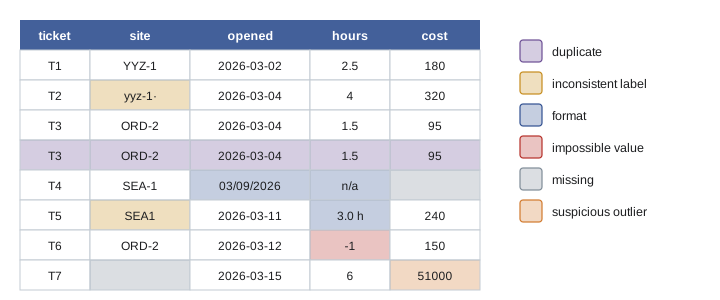
Cleaning with explicit decisions

Each problem needs a decision, and each decision should be visible in the code:

• Duplicates: exact duplicate rows are usually safe to drop. Rows that share an ID but differ elsewhere need investigation: which version is correct?
• Inconsistent labels: strip whitespace, standardize case, and map known variants to a canonical form. For large category sets, keep an explicit mapping table and report any values not in it.
• Numbers stored as text: remove units or symbols, then convert with pd.to_numeric(..., errors="coerce"), which turns anything unparseable into NaN so that it can be counted rather than crashing the program.
• Impossible values: negative repair hours, temperatures of −40 °C inside a data hall, or dates in the future are errors. Convert them to missing (or fix them from the source) and record how many there were.
• Dates: parse with an explicit format. Mixed formats need special care.

import pandas as pd

raw = pd.DataFrame({
    "ticket": ["T1", "T2", "T3", "T3", "T4", "T5", "T6", "T7"],
    "site": ["YYZ-1", "yyz-1 ", "ORD-2", "ORD-2", "SEA-1", "SEA1", "ORD-2", None],
    "opened": ["2026-03-02", "2026-03-04", "2026-03-04", "2026-03-04", "03/09/2026", "2026-03-11", "2026-03-12", "2026-03-15"],
    "hours": ["2.5", "4", "1.5", "1.5", "n/a", "3.0 h", "-1", "6"],
    "cost": [180.0, 320.0, 95.0, 95.0, None, 240.0, 150.0, 51000.0],
})

df = raw.drop_duplicates().copy()
df["site"] = (df["site"].str.strip().str.upper()
              .str.replace("SEA1", "SEA-1", regex=False))
df["hours"] = pd.to_numeric(df["hours"].str.replace(" h", "", regex=False), errors="coerce")
df.loc[df["hours"] < 0, "hours"] = float("nan")          # impossible values become missing
df["opened"] = pd.to_datetime(df["opened"], format="ISO8601", errors="coerce")

print(df.to_string(index=False))
print("Unparsed dates:", df["opened"].isna().sum(), "| missing hours:", df["hours"].isna().sum())

ticket  site     opened  hours    cost
    T1 YYZ-1 2026-03-02    2.5   180.0
    T2 YYZ-1 2026-03-04    4.0   320.0
    T3 ORD-2 2026-03-04    1.5    95.0
    T4 SEA-1        NaT    NaN     NaN
    T5 SEA-1 2026-03-11    3.0   240.0
    T6 ORD-2 2026-03-12    NaN   150.0
    T7   NaN 2026-03-15    6.0 51000.0
Unparsed dates: 1 | missing hours: 2

The cleaned table still has gaps, and that is correct: it now shows honestly what is known and what is not. Note how the date "03/09/2026" was not parsed. That is deliberate: in Canada and much of the world it would normally mean 3 September, and in the United States 9 March. Guessing silently would put the ticket in the wrong month half the time. The right fix is to find out from the source system which format it used, and in the future to insist on ISO 8601 dates (Lesson 2).

Missing data

Lesson 5 introduced pandas' tools for missing values: isna, dropna and fillna. The harder question is why data is missing, because the reason decides what is safe to do:

• Missing completely at random: a sensor occasionally drops a reading for reasons unrelated to anything else. Dropping or simple filling causes little bias.
• Missing at random, given other variables: costs are more often missing for tickets from one site whose system does not record them. Filling within groups, or modeling the missing values from other columns, can work.
• Missing not at random: the missingness depends on the missing value itself. Temperatures go missing when a sensor overheats and shuts down, so the hottest readings are exactly the ones lost. Any simple fill will understate the problem.

Common strategies are to drop rows (simple, but loses data and can bias results), fill with a constant, the median or a group median, interpolate in time series (Lesson 5), or keep a separate indicator column saying the value was missing, which lets a model learn whether missingness itself is informative. Whatever you choose, report how many values were missing and what you did.

Outliers

An outlier is a value far from the rest. It may be an error (a stuck sensor reading 85 °C), a real but rare event (a genuine hot spot of 41.5 °C) or simply the tail of a skewed distribution (a long repair). The aim is to detect outliers, then decide what each one is.

• The IQR rule flags values below Q1 − 1.5 IQR or above Q3 + 1.5 IQR, where IQR = Q3 − Q1 is the interquartile range. It is the rule behind box plots (Lesson 7).
• The z-score \(z = (x - \bar{x})/s\) flags values more than about 3 standard deviations from the mean. But outliers inflate the mean and standard deviation themselves, which can hide other outliers.
• The robust z-score uses the median and the median absolute deviation (MAD) instead, which outliers barely affect: \(z_{r} = 0.6745\,(x - \tilde{x})/\text{MAD}\), flagging values with \(|z_{r}| > 3.5\).

import numpy as np
import pandas as pd

rng = np.random.default_rng(5)
inlet = pd.Series(np.round(rng.normal(24.0, 1.2, 200), 1))
inlet.iloc[[17, 88, 150]] = [41.5, 85.0, -40.0]     # a hot spot, a stuck sensor, a disconnected probe

q1, q3 = inlet.quantile([0.25, 0.75])
iqr = q3 - q1
iqr_flags = (inlet < q1 - 1.5 * iqr) | (inlet > q3 + 1.5 * iqr)

z = (inlet - inlet.mean()) / inlet.std()
med = inlet.median()
mad = (inlet - med).abs().median()
robust_z = 0.6745 * (inlet - med) / mad

print(f"IQR fences: {q1 - 1.5 * iqr:.1f} to {q3 + 1.5 * iqr:.1f} C, flagged {iqr_flags.sum()}")
print("Ordinary z > 3:", int((z.abs() > 3).sum()), "| robust z > 3.5:", int((robust_z.abs() > 3.5).sum()))
print(pd.DataFrame({"value": inlet, "z": z.round(1), "robust_z": robust_z.round(1)})[iqr_flags].to_string())

IQR fences: 20.5 to 27.2 C, flagged 3
Ordinary z > 3: 2 | robust z > 3.5: 3
     value    z  robust_z
17    41.5  2.7      14.0
88    85.0  9.4      48.5
150  -40.0 -9.9     -50.7

The ordinary z-score missed the 41.5 °C hot spot (z = 2.7), because the two extreme sensor errors inflated the standard deviation. The IQR rule and the robust z-score caught all three. Having found them, the analyst should treat them differently: the 85 °C and −40 °C values are sensor faults to be removed, but the 41.5 °C reading may be the most important number in the data set, a real hot spot that needs attention.

Preparing features for machine learning

Machine learning models need numeric inputs, called features. Preparing them is called feature engineering. Common steps are:

• Encoding categories: one-hot encoding turns a column with values air, liquid and hybrid into three 0/1 columns. Avoid simply numbering categories 1, 2, 3, which implies an order and spacing that does not exist.
• Scaling: many models work better when numeric features have similar ranges. Standardization subtracts the mean and divides by the standard deviation; min-max scaling maps values to 0–1.
• Transforming: logarithms tame skewed quantities such as costs and durations; dates become features such as hour of day, day of week or month.
• Combining: ratios and differences, such as power per rack or the difference between supply and return temperature, often carry more information than the raw columns.

Data leakage

The most damaging preparation mistake is leakage: letting information from the test data, or from the future, into the training process. A model evaluated on data it has effectively seen will look better than it really is, and will disappoint in use. Scaling is a classic source: if the mean and standard deviation are computed from the whole data set before splitting it into training and test sets, the test set has influenced the training. The rule is to split first, then compute every statistic, encoding and fill value from the training data only, and apply them unchanged to the test data.

import numpy as np
import pandas as pd

rng = np.random.default_rng(8)
n = 10
df = pd.DataFrame({
    "cooling": rng.choice(["air", "liquid", "hybrid"], n),
    "it_kw": np.round(rng.uniform(5, 60, n), 1),
    "outside_c": np.round(rng.uniform(-20, 35, n), 1),
})

encoded = pd.get_dummies(df, columns=["cooling"], dtype=int)
print(encoded.head(3).to_string(index=False))

train, test = encoded.iloc[:7], encoded.iloc[7:]
mu, sd = train["it_kw"].mean(), train["it_kw"].std()
train_scaled = (train["it_kw"] - mu) / sd
test_scaled = (test["it_kw"] - mu) / sd          # use training statistics only
print(f"Training mean {mu:.1f} kW, sd {sd:.1f} kW")
print("Scaled test values:", test_scaled.round(2).tolist())

 it_kw  outside_c  cooling_air  cooling_hybrid  cooling_liquid
  26.5        3.3            0               1               0
  29.1       -5.9            1               0               0
  25.5       12.5            1               0               0
Training mean 23.0 kW, sd 7.2 kW
Scaled test values: [-1.08, -1.01, 3.74]

The last test value scales to 3.74: it is far above anything in the training data, and the model will be extrapolating there. Using training statistics makes that visible instead of hiding it. Other common forms of leakage include features that are recorded only after the outcome (such as "repair cost" when predicting whether a failure will occur), random splits of time series that let a model train on the future, and duplicates that land in both training and test sets. Lesson 9 shows how scikit-learn pipelines prevent most of these mistakes automatically.

Validating every batch

Data pipelines run again and again on new data, and upstream systems change without warning: a column is renamed, a unit changes from kW to W, a new site appears with a new code. Automated validation checks every batch against expectations before it is used, and stops the pipeline loudly instead of letting bad data flow quietly into reports and models.

import pandas as pd

def validate(df):
    problems = []
    required = {"ticket", "site", "hours", "cost"}
    if missing := required - set(df.columns):
        problems.append(f"missing columns {sorted(missing)}")
    if df["ticket"].duplicated().any():
        problems.append("duplicate ticket IDs")
    bad_hours = df["hours"].lt(0) | df["hours"].gt(72)
    if bad_hours.any():
        problems.append(f"{bad_hours.sum()} hours outside 0-72")
    share_missing = df["cost"].isna().mean()
    if share_missing > 0.10:
        problems.append(f"cost missing in {share_missing:.0%} of rows")
    return problems

batch = pd.DataFrame({"ticket": ["T8", "T9", "T9"], "site": ["YYZ-1", "SEA-1", "SEA-1"],
                      "hours": [3.0, 96.0, 2.0], "cost": [210.0, None, 140.0]})
issues = validate(batch)
print("PASS" if not issues else "FAIL: " + "; ".join(issues))

FAIL: duplicate ticket IDs; 1 hours outside 0-72; cost missing in 33% of rows

Checks like these can be written by hand, as here, or with libraries such as pandera and Great Expectations, which let you declare a schema of column names, types, ranges and allowed values. Validation rules are also documentation: they record what the team believes about the data, and a failing rule is often the first sign that something upstream has changed.

Keep a cleaning log

Every cleaning decision changes the results, so it must be reproducible and reviewable. Keep the raw data unchanged, do all cleaning in code (never by hand-editing files), and record the decisions with counts: "dropped 1 duplicate; standardized 5 site spellings to 3 sites; 1 date in ambiguous format left missing pending confirmation; 1 negative hours value set to missing; 1 cost of $51,000 flagged for review." Such a log lets others check your work and lets you rerun everything when the data is updated (Lesson 11).