Data frames with pandas

Most data that feeds AI systems arrives as tables: rows of records with named columns of different types. A table of customers has names (text), sign-up dates (dates), plans (categories) and monthly spend (numbers). A log of sensor readings has timestamps, device identifiers and measurements. NumPy arrays hold one type of number in a grid; they have no column names, no mixed types and no natural way to handle dates or missing values. For tables, Python has pandas.

Pandas provides the DataFrame, a table with labeled rows and columns in which each column can have its own type, and a large set of tools to load, clean, filter, combine, group, summarize and reshape such tables. Industry surveys consistently rank it among the most used tools in data science, and in practice a large share of any AI project's time goes into exactly this kind of data preparation. This chapter covers the operations you will use every day. The examples use pandas 2.2 or later; text columns appear as "object" in pandas 2 and as "str" in pandas 3, but everything shown works the same in both.

Series and DataFrames

Pandas has two main objects:

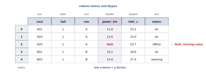
• A Series is a one-dimensional array of values with an index (labels for each value). It is like a NumPy array with names attached, and it is what you get when you select one column of a table.
• A DataFrame is a two-dimensional table: a collection of Series sharing the same index, one per column. Each column has a name and a dtype.

The index labels the rows. By default it is simply 0, 1, 2 and so on, but it can be anything meaningful, such as rack identifiers or timestamps. Labels let pandas align data automatically: when two Series are added, values are matched by label, not by position.

Loading data

Pandas reads data from many formats: pd.read_csv for comma-separated text, pd.read_excel for spreadsheets, pd.read_json, pd.read_parquet for the efficient columnar format used in data engineering, and pd.read_sql for databases. CSV is the most common. The example below reads a small CSV of rack measurements from a string (via io.StringIO, which makes a string behave like a file) so that the program is self-contained; with a real file you would write pd.read_csv("racks.csv").

import io
import pandas as pd

csv_text = """rack,hall,row,power_kw,inlet_c,status
A01,1,A,11.8,23.1,ok
A02,1,A,12.6,24.0,ok
A03,1,A,,23.7,offline
B01,1,B,15.2,26.8,ok
B02,1,B,14.9,27.4,warning
C01,2,C,9.4,21.9,ok
C02,2,C,10.1,22.5,ok
C03,2,C,18.7,28.9,warning
"""
df = pd.read_csv(io.StringIO(csv_text))
print(df.shape)
print(df.head(3))
print(df["power_kw"].describe().round(2))

(8, 6)
  rack  hall row  power_kw  inlet_c   status
0  A01     1   A      11.8     23.1       ok
1  A02     1   A      12.6     24.0       ok
2  A03     1   A       NaN     23.7  offline
count     7.00
mean     13.24
std       3.25
min       9.40
25%      10.95
50%      12.60
75%      15.05
max      18.70
Name: power_kw, dtype: float64

The first look at any new data set follows the same routine: df.shape for the number of rows and columns, df.head() to see a few rows, df.info() for column types and non-missing counts, and df.describe() for summary statistics of numeric columns. Notice that read_csv did several things automatically. It used the first line as column names, worked out that hall is an integer and power_kw a float, and turned the empty power_kw value for rack A03 into NaN ("not a number"), pandas' marker for a missing value. The count of 7 in describe() shows that one of the eight values is missing and was left out of the statistics.

Selecting, filtering and new columns

Pandas offers several ways to select data, and it is worth learning the clear, explicit ones:

• df["power_kw"] selects one column as a Series; df[["rack", "power_kw"]] (note the double brackets) selects several columns as a DataFrame.
• df.loc[rows, columns] selects by label: df.loc[3, "inlet_c"], or df.loc[df["hall"] == 2, ["rack", "inlet_c"]].
• df.iloc[rows, columns] selects by integer position, like NumPy: df.iloc[0:3, 1:4].
• A Boolean mask in brackets filters rows: df[df["inlet_c"] > 25].

New columns are created by assigning a vectorized expression, exactly as with NumPy arrays.

import io
import pandas as pd

df = pd.read_csv(io.StringIO("""rack,hall,row,power_kw,inlet_c,status
A01,1,A,11.8,23.1,ok
A02,1,A,12.6,24.0,ok
A03,1,A,,23.7,offline
B01,1,B,15.2,26.8,ok
B02,1,B,14.9,27.4,warning
C01,2,C,9.4,21.9,ok
C02,2,C,10.1,22.5,ok
C03,2,C,18.7,28.9,warning
"""))
hot = df[df["inlet_c"] > 25]                      # filter rows with a mask
print(hot[["rack", "power_kw", "inlet_c"]])
df["inlet_f"] = df["inlet_c"] * 9 / 5 + 32        # new column, vectorized
print(df.loc[df["hall"] == 2, ["rack", "inlet_f"]])
print(df.sort_values("power_kw", ascending=False).head(3)["rack"].tolist())

  rack  power_kw  inlet_c
3  B01      15.2     26.8
4  B02      14.9     27.4
7  C03      18.7     28.9
  rack  inlet_f
5  C01    71.42
6  C02    72.50
7  C03    84.02
['C03', 'B01', 'B02']

Filtering keeps the original index labels (3, 4 and 7), which tells you where each row came from. Conditions combine with & and |, with parentheses around each one, as in NumPy: df[(df["hall"] == 1) & (df["status"] != "ok")]. The method df.query("inlet_c > 25 and hall == 1") expresses the same thing as a readable string.

Grouping and aggregation

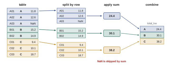
Many questions about data take the form "for each group, compute something": total power per row, average temperature per hall, number of alarms per day. Pandas answers them with groupby, which follows a pattern called split-apply-combine: split the rows into groups by the values of one or more columns, apply a summary function to each group, and combine the results into a new table.

import io
import pandas as pd

df = pd.read_csv(io.StringIO("""rack,hall,row,power_kw,inlet_c,status
A01,1,A,11.8,23.1,ok
A02,1,A,12.6,24.0,ok
A03,1,A,,23.7,offline
B01,1,B,15.2,26.8,ok
B02,1,B,14.9,27.4,warning
C01,2,C,9.4,21.9,ok
C02,2,C,10.1,22.5,ok
C03,2,C,18.7,28.9,warning
"""))
by_row = df.groupby("row").agg(racks=("rack", "count"),
                               total_kw=("power_kw", "sum"),
                               max_inlet=("inlet_c", "max"))
print(by_row)
print(df.groupby("hall")["power_kw"].mean().round(2))
print(df["status"].value_counts())

     racks  total_kw  max_inlet
row
A        3      24.4       24.0
B        2      30.1       27.4
C        3      38.2       28.9
hall
1    13.62
2    12.73
Name: power_kw, dtype: float64
status
ok         5
warning    2
offline    1
Name: count, dtype: int64

The agg method with named aggregations (new_name=(column, function)) produces tidy, clearly labeled results. Note that row A has 3 racks but its total uses only the two with readings, because sum skips NaN. The hall 1 mean of 13.62 kW is likewise the average of the four racks with readings, not five. value_counts is the quickest way to see how often each category occurs, and it is one of the first things to run on any categorical column.

Missing data

Missing values are the norm in real data: sensors fail, forms are left incomplete, systems are offline. Pandas represents them as NaN for numbers (and NaT for missing dates), and provides tools to find and handle them (Lesson 6 discusses how to decide which to use):

• df.isna() returns a mask of missing values; df.isna().sum() counts them per column.
• df.dropna() removes rows with missing values (subset= restricts which columns to check).
• df.fillna(value) replaces missing values, for example with a constant, a column mean or the previous value (ffill).
• s.interpolate() estimates missing values in a series from their neighbors, which suits smoothly varying measurements over time.

import io
import pandas as pd

df = pd.read_csv(io.StringIO("""rack,hall,row,power_kw,inlet_c,status
A01,1,A,11.8,23.1,ok
A02,1,A,12.6,24.0,ok
A03,1,A,,23.7,offline
B01,1,B,15.2,26.8,ok
"""))
print(df["power_kw"].isna().sum(), "missing")
print(round(df["power_kw"].mean(), 2))             # NaN is skipped
print(round(df["power_kw"].fillna(0).mean(), 2))   # treating missing as zero
print(df.dropna(subset=["power_kw"])["rack"].tolist())

1 missing
13.2
9.9
['A01', 'A02', 'B01']

The two means differ by a third, which shows why the choice matters. There is no universally right answer: it depends on why the data is missing. If the rack is offline, zero is correct for energy totals; if its meter failed while the rack ran normally, zero badly understates the load and skipping or interpolating is better. Whatever you choose, make it a deliberate decision, write it down, and check how much it changes the results. In machine learning, how missing values are filled can also leak information or bias a model, a topic covered in AI-220.

Combining tables

Data usually lives in several tables that must be joined: measurements in one, equipment details in another, customer information in a third. The merge method joins two DataFrames on matching key columns, like a database join:

• how="inner" keeps only rows whose key appears in both tables.
• how="left" keeps every row of the left table, filling NaN where the right table has no match.
• how="outer" keeps every row from both.

import pandas as pd

racks = pd.DataFrame({"rack": ["A01", "A02", "B01", "C01"],
                      "customer_id": [7, 7, 12, 31],
                      "power_kw": [11.8, 12.6, 15.2, 9.4]})
customers = pd.DataFrame({"customer_id": [7, 12, 40],
                          "name": ["Northwind", "Bluebird AI", "Cedar Labs"]})
merged = racks.merge(customers, on="customer_id", how="left")
print(merged)
print(merged.groupby("name")["power_kw"].sum())

  rack  customer_id  power_kw         name
0  A01            7      11.8    Northwind
1  A02            7      12.6    Northwind
2  B01           12      15.2  Bluebird AI
3  C01           31       9.4          NaN
name
Bluebird AI    15.2
Northwind      24.4
Name: power_kw, dtype: float64

Rack C01 belongs to customer 31, who is missing from the customer table, so the left join gives it a NaN name, and the groupby then drops it from the totals without any warning. A careful analyst checks for unmatched keys after every merge (for example with merged["name"].isna().sum()) because a silent loss of rows like this is one of the most common causes of wrong numbers in reports. The validate argument of merge can also enforce expectations, such as each rack matching at most one customer. pd.concat, by contrast, stacks tables with the same columns on top of each other, for example a month of daily files.

Time series

Measurements over time are central to engineering and AI: sensor logs, energy use, transactions, web traffic. Pandas has strong support for them. pd.to_datetime converts text to timestamps; pd.date_range creates regular sequences of times; and a Series or DataFrame with a DatetimeIndex gains time-aware tools. resample changes the frequency (hourly to daily, for example) with an aggregation, and rolling computes moving-window statistics such as a 24-hour moving average.

import numpy as np
import pandas as pd

rng = np.random.default_rng(1)
times = pd.date_range("2026-07-01", periods=7 * 24, freq="h")    # one week, hourly
hours = times.hour.to_numpy()
load = 800 + 120 * np.sin((hours - 9) / 24 * 2 * np.pi) + rng.normal(0, 15, len(times))
s = pd.Series(load, index=times, name="it_load_kw")

daily = s.resample("D").agg(["mean", "max"]).round(1)
print(daily.head(3))
print(s.rolling(24).mean().dropna().round(1).iloc[:2])
print("peak hour:", s.idxmax())

             mean    max
2026-07-01  801.7  929.0
2026-07-02  796.2  921.6
2026-07-03  799.3  918.9
2026-07-01 23:00:00    801.7
2026-07-02 00:00:00    799.8
Freq: h, Name: it_load_kw, dtype: float64
peak hour: 2026-07-07 16:00:00

The program simulates a week of hourly IT load with a daily cycle (peaking in the afternoon) plus random noise. Resampling to daily frequency gives each day's mean and peak. The 24-hour rolling mean needs 24 values before it can produce its first result, so the first 23 entries are NaN, which dropna removes; the first full window ends at 23:00 on 1 July. Rolling means smooth out the daily cycle to reveal longer trends, a standard first step before forecasting.

Tidy data and method chaining

Analysis is easiest when data is "tidy": each variable is a column, each observation is a row, and each kind of observational unit is its own table. A spreadsheet with one column per month is not tidy, because the month is a variable hiding in the column names; df.melt reshapes it into long form with a month column and a value column, and df.pivot_table reshapes the other way for reports. Pandas code is also often written as a chain of methods, one per line, which reads like a recipe:

• (df.query("status == 'ok'").groupby("row")["power_kw"].sum().sort_values(ascending=False))

Each step returns a new DataFrame, so the original is unchanged, and the chain documents exactly how a result was produced.

Performance and scale

Pandas keeps the whole table in memory and works best on data up to a few gigabytes. As with NumPy, vectorized column operations are fast and row-by-row loops (iterrows, or apply with a Python function) are slow, so prefer column expressions. For larger data, the Parquet file format loads faster and smaller than CSV, and libraries such as Polars, DuckDB and Spark handle data sets that are too large or too slow for pandas while keeping similar ideas.