Databases, SQL and data at scale

Most of the data an organization owns does not live in CSV files. It lives in databases: the ticketing system, the asset inventory, the billing platform, the building management system's history, the data warehouse that combines them. To work with that data you need SQL (Structured Query Language), the language almost every database speaks, and you need to know how to move data efficiently between databases and Python. This lesson introduces relational databases and SQL using SQLite, which is built into Python, shows how pandas reads query results, and covers the techniques for data too large to load at once and for collecting data from web APIs.

Relational databases

A relational database stores data in tables of rows and columns, much like DataFrames, but with important differences:

• Each table has a fixed schema: column names and types are declared in advance and enforced.
• A primary key uniquely identifies each row (a site ID, an incident number).
• Foreign keys link tables: each incident row stores the site_id of the site it belongs to, rather than repeating the site's city and capacity. This avoids duplicated, inconsistent data, a design principle called normalization.
• The database enforces rules, handles many users at once, and guarantees that a transaction (a group of changes) either completes entirely or not at all.

Common systems include PostgreSQL, MySQL and MariaDB, Microsoft SQL Server and Oracle for applications; SQLite for embedded and local use; and cloud data warehouses such as Snowflake, Google BigQuery, Amazon Redshift and Databricks for analytics over very large data.

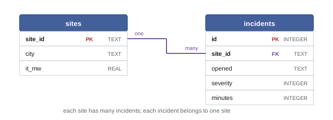
Creating and querying tables

SQL statements read almost like English. CREATE TABLE defines a table; INSERT adds rows; SELECT ... FROM ... WHERE ... ORDER BY retrieves them.

import sqlite3

con = sqlite3.connect(":memory:")          # a throwaway database in memory
con.executescript("""
CREATE TABLE sites (site_id TEXT PRIMARY KEY, city TEXT, it_mw REAL);
CREATE TABLE incidents (
    id INTEGER PRIMARY KEY,
    site_id TEXT REFERENCES sites(site_id),
    opened TEXT,
    severity INTEGER,
    minutes INTEGER
);
""")
con.executemany("INSERT INTO sites VALUES (?, ?, ?)",
                [("YYZ-1", "Toronto", 36.0), ("ORD-2", "Chicago", 48.0), ("SEA-1", "Seattle", 24.0)])
con.executemany("INSERT INTO incidents (site_id, opened, severity, minutes) VALUES (?, ?, ?, ?)", [
    ("YYZ-1", "2026-09-02", 2, 45), ("YYZ-1", "2026-09-19", 1, 210), ("ORD-2", "2026-09-05", 3, 15),
    ("ORD-2", "2026-09-21", 2, 60), ("ORD-2", "2026-10-01", 2, 35), ("SEA-1", "2026-09-30", 3, 20),
])
con.commit()

rows = con.execute(
    "SELECT site_id, opened, minutes FROM incidents WHERE severity <= ? ORDER BY minutes DESC",
    (2,),
).fetchall()
for r in rows:
    print(r)

('YYZ-1', '2026-09-19', 210)
('ORD-2', '2026-09-21', 60)
('YYZ-1', '2026-09-02', 45)
('ORD-2', '2026-10-01', 35)

Notice the question marks. Values are never pasted into SQL text; they are passed separately as parameters, and the database inserts them safely. This matters enormously for security. If a program builds SQL by joining strings, a value supplied by a user, such as a site name typed into a form, can contain SQL code that the database will run. This attack, SQL injection, has been behind many of the largest data breaches. Parameterized queries make it impossible, because the database always treats parameters as data, never as code.

Aggregating and joining

SQL's real power is in combining and summarizing. GROUP BY with aggregate functions (COUNT, SUM, AVG, MIN, MAX) summarizes groups, exactly like pandas groupby (Lesson 5). JOIN combines tables on matching keys, like pandas merge:

• INNER JOIN keeps only rows with a match in both tables.
• LEFT JOIN keeps every row of the left table, filling missing matches with NULL.

import sqlite3

con = sqlite3.connect(":memory:")
con.executescript("""
CREATE TABLE sites (site_id TEXT PRIMARY KEY, city TEXT, it_mw REAL);
CREATE TABLE incidents (id INTEGER PRIMARY KEY, site_id TEXT, opened TEXT, severity INTEGER, minutes INTEGER);
""")
con.executemany("INSERT INTO sites VALUES (?, ?, ?)",
                [("YYZ-1", "Toronto", 36.0), ("ORD-2", "Chicago", 48.0), ("SEA-1", "Seattle", 24.0), ("YUL-3", "Montreal", 12.0)])
con.executemany("INSERT INTO incidents (site_id, opened, severity, minutes) VALUES (?, ?, ?, ?)", [
    ("YYZ-1", "2026-09-02", 2, 45), ("YYZ-1", "2026-09-19", 1, 210), ("ORD-2", "2026-09-05", 3, 15),
    ("ORD-2", "2026-09-21", 2, 60), ("ORD-2", "2026-10-01", 2, 35), ("SEA-1", "2026-09-30", 3, 20),
])

query = """
SELECT s.site_id, s.city,
       COUNT(i.id)                 AS incidents,
       COALESCE(SUM(i.minutes), 0) AS total_minutes,
       ROUND(COUNT(i.id) / s.it_mw * 10, 2) AS per_10_mw
FROM sites AS s
LEFT JOIN incidents AS i ON i.site_id = s.site_id
GROUP BY s.site_id
ORDER BY per_10_mw DESC
"""
for row in con.execute(query):
    print(row)

('ORD-2', 'Chicago', 3, 110, 0.63)
('YYZ-1', 'Toronto', 2, 255, 0.56)
('SEA-1', 'Seattle', 1, 20, 0.42)
('YUL-3', 'Montreal', 0, 0, 0.0)

Two details deserve attention. The LEFT JOIN keeps Montreal, which had no incidents; an inner join would have dropped it silently, making the list look as if Montreal did not exist rather than having a perfect record. And COALESCE replaces the NULL sum for that site with 0. Normalizing by size (incidents per 10 MW of IT load) makes sites of different sizes comparable, a theme from Lesson 8.

SQL and pandas together

pandas reads query results straight into a DataFrame with pd.read_sql_query, and writes DataFrames to tables with to_sql. A good rule of thumb is to let the database do the filtering, joining and aggregating, which it does efficiently next to the data, and bring only the result into Python for analysis, modeling and plotting. Pulling an entire billion-row table into pandas to filter it there is slow and often impossible.

Modern SQL also offers window functions, which compute values across related rows without collapsing them into groups: running totals, rankings, moving averages and comparisons with the previous row.

import sqlite3
import pandas as pd

con = sqlite3.connect(":memory:")
pd.DataFrame({
    "site_id": ["YYZ-1", "YYZ-1", "ORD-2", "ORD-2", "ORD-2", "SEA-1"],
    "opened": ["2026-09-02", "2026-09-19", "2026-09-05", "2026-09-21", "2026-10-01", "2026-09-30"],
    "minutes": [45, 210, 15, 60, 35, 20],
}).to_sql("incidents", con, index=False)

df = pd.read_sql_query(
    "SELECT site_id, opened, minutes, "
    "SUM(minutes) OVER (PARTITION BY site_id ORDER BY opened) AS running_minutes "
    "FROM incidents WHERE opened >= ? ORDER BY site_id, opened",
    con, params=("2026-09-01",), parse_dates=["opened"])
print(df.to_string(index=False))
print(df.dtypes["opened"])

site_id     opened  minutes  running_minutes
  ORD-2 2026-09-05       15               15
  ORD-2 2026-09-21       60               75
  ORD-2 2026-10-01       35              110
  SEA-1 2026-09-30       20               20
  YYZ-1 2026-09-02       45               45
  YYZ-1 2026-09-19      210              255
datetime64[us]

The parse_dates argument converts the text dates into proper datetime values on the way in. SQLite stores dates as text, so date comparisons such as opened >= ? work only because ISO 8601 strings sort in date order, one more reason to use that format everywhere (Lesson 2).

Data too big for memory

A DataFrame lives entirely in memory, and pandas typically needs several times the size of the data while working on it. When files grow to many gigabytes, three techniques help before you need different tools:

• Choose compact types: categorical columns for repeated text, float32 instead of float64 where precision allows, and only the columns you need (usecols).
• Process in chunks: read_csv(..., chunksize=n) returns the file in pieces, so you can aggregate as you go.
• Use better file formats: Parquet stores each column compressed and typed, so it is smaller and much faster to read, and you can read only the columns you need.

import numpy as np
import pandas as pd

rng = np.random.default_rng(6)
n = 200_000
pd.DataFrame({
    "rack": rng.choice([f"R{i:03d}" for i in range(400)], n),
    "status": rng.choice(["ok", "warn", "alarm"], n, p=[0.97, 0.025, 0.005]),
    "kw": rng.normal(12, 3, n).round(2),
}).to_csv("telemetry.csv", index=False)

full = pd.read_csv("telemetry.csv")
print(f"As read: {full.memory_usage(deep=True).sum() / 1e6:.1f} MB")
slim = pd.read_csv("telemetry.csv", dtype={"rack": "category", "status": "category", "kw": "float32"})
print(f"With categories and float32: {slim.memory_usage(deep=True).sum() / 1e6:.1f} MB")

alarms = 0
for chunk in pd.read_csv("telemetry.csv", chunksize=50_000):
    alarms += (chunk["status"] == "alarm").sum()
print("Alarms counted in 4 chunks:", alarms)

As read: 22.4 MB
With categories and float32: 1.4 MB
Alarms counted in 4 chunks: 1044

Declaring the repeated rack and status strings as categories, and the power as float32, cut memory use from about 22 MB to about 1.4 MB, a factor of 16. The same idea applied to a 20 GB file can be the difference between needing a cluster and running on a laptop.

Beyond that, specialized tools take over. Polars and DuckDB are fast, memory-efficient libraries for single machines that can query files larger than memory; DuckDB runs SQL directly on CSV and Parquet files. Apache Spark and Dask spread work across many machines. Cloud data warehouses run SQL on petabytes. The concepts of this course, tables, filtering, grouping, joining and tidy data, carry over to all of them.

Collecting data from web APIs

Many data sources, such as weather services, cloud billing, monitoring platforms and ticketing systems, offer web APIs that return JSON (Lesson 2). Code that collects from them must handle a few realities:

• Authentication: requests carry an API key or token, which must be kept out of code and notebooks, in environment variables or a secrets manager.
• Pagination: large results come back one page at a time, with a link or token for the next page.
• Rate limits: services cap requests per minute and reply with an error (HTTP 429) when exceeded.
• Transient failures: networks fail occasionally, so code should retry with exponential backoff, waiting longer after each failure, and give up cleanly after a few tries.

import time

DATA = [{"id": i, "kw": round(5 + (i * 37 % 100) / 10, 1)} for i in range(1, 24)]
calls = {"n": 0}

def fake_api(page, size=10):
    """Pretend web API: returns one page of results; fails on the 2nd call."""
    calls["n"] += 1
    if calls["n"] == 2:
        raise ConnectionError("temporary network error")
    start = (page - 1) * size
    items = DATA[start:start + size]
    return {"items": items, "next_page": page + 1 if start + size < len(DATA) else None}

def fetch_all(max_retries=3):
    page, results = 1, []
    while page is not None:
        for attempt in range(1, max_retries + 1):
            try:
                reply = fake_api(page)
                break
            except ConnectionError as err:
                wait = 0.01 * 2 ** attempt
                print(f"page {page}: {err}; retrying in {wait:.2f} s")
                time.sleep(wait)
        else:
            raise RuntimeError(f"gave up on page {page}")
        results.extend(reply["items"])
        page = reply["next_page"]
    return results

rows = fetch_all()
print(len(rows), "records in", calls["n"], "calls; last:", rows[-1])

page 2: temporary network error; retrying in 0.02 s
23 records in 4 calls; last: {'id': 23, 'kw': 10.1}

Real code would use a library such as requests or httpx to make the HTTP calls, but the structure is the same: loop over pages, retry failures with increasing waits, stop when there is no next page, and save the raw responses before transforming them, so that a bug in the transformation never forces you to download everything again. Respect each service's terms of use and rate limits.

When collecting data about people, US privacy laws, which vary by sector and by state (such as the California Consumer Privacy Act), set rules on notice, use and safeguards; collect only what you need.